# Technical Analysis: Mixture-of-Depths Performance vs. Baseline
This document provides a detailed extraction of data and trends from a two-panel technical visualization comparing "Baseline" models to "Mixture-of-Depths" (MoD) models across various compute budgets and parameter scales.
---
## 1. Left Panel: Loss vs. Parameters by FLOP Budget
### Axis and Labels
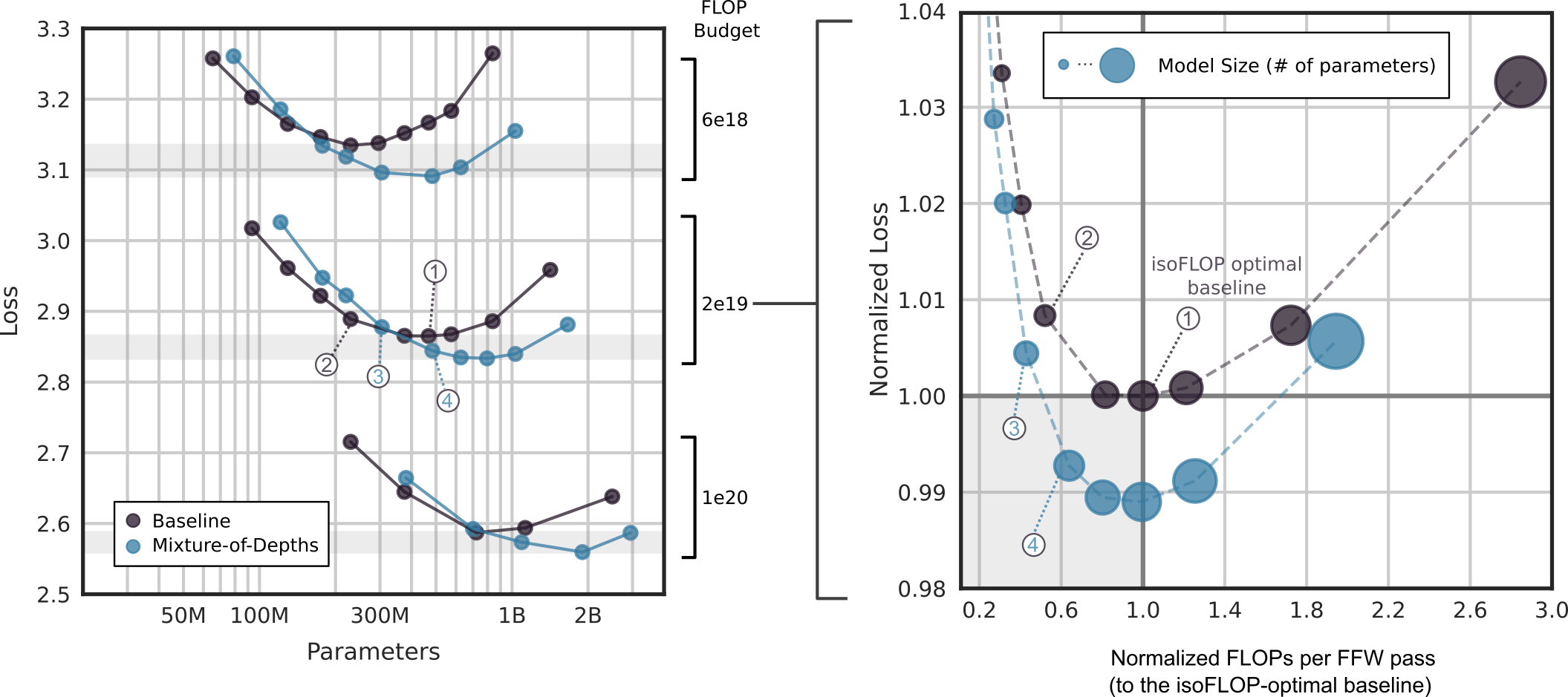
* **Y-Axis:** Loss (Linear scale from 2.5 to 3.3).
* **X-Axis:** Parameters (Logarithmic scale: 50M, 100M, 300M, 1B, 2B).
* **Legend (Bottom Left):**
* **Dark Purple Circle:** Baseline
* **Light Blue Circle:** Mixture-of-Depths
* **Right-side Labels (FLOP Budget):** Brackets indicate three distinct compute tiers:
* **6e18** (Top tier)
* **2e19** (Middle tier)
* **1e20** (Bottom tier)
### Data Trends and Observations
The chart displays three pairs of curves, one pair for each FLOP budget. Each curve follows a U-shape, indicating an optimal parameter count for a fixed compute budget.
#### Tier 1: 6e18 FLOPs (Top Curves)
* **Baseline (Purple):** Slopes downward to a minimum near 300M parameters (Loss ~3.13), then slopes upward toward 1B.
* **Mixture-of-Depths (Blue):** Slopes downward to a minimum near 500M parameters (Loss ~3.09), then slopes upward.
* **Key Finding:** MoD achieves a lower minimum loss than the baseline and shifts the optimal parameter count to the right (larger model).
#### Tier 2: 2e19 FLOPs (Middle Curves)
* **Baseline (Purple):** Minimum loss (~2.86) occurs around 500M-700M parameters.
* **Mixture-of-Depths (Blue):** Minimum loss (~2.83) occurs around 1B parameters.
* **Callouts:**
* Point **(1)** identifies the baseline minimum.
* Point **(2)** identifies a smaller baseline model.
* Point **(3)** identifies a smaller MoD model.
* Point **(4)** identifies the MoD minimum.
#### Tier 3: 1e20 FLOPs (Bottom Curves)
* **Baseline (Purple):** Minimum loss (~2.59) occurs around 1B parameters.
* **Mixture-of-Depths (Blue):** Minimum loss (~2.56) occurs around 2B parameters.
---
## 2. Right Panel: Normalized Loss vs. Normalized FLOPs
This panel aggregates the data to show efficiency relative to the "isoFLOP optimal baseline."
### Axis and Labels
* **Y-Axis:** Normalized Loss (Linear scale from 0.98 to 1.04).
* **X-Axis:** Normalized FLOPs per FFW pass (to the isoFLOP-optimal baseline) (Linear scale from 0.2 to 3.0).
* **Legend (Top):**
* **Circle Size:** Represents Model Size (# of parameters). Larger circles = more parameters.
* **Dashed Lines:** Connect data points of the same type.
* **Reference Lines:**
* **Horizontal line at 1.00:** Represents the loss of the optimal baseline.
* **Vertical line at 1.0:** Represents the FLOP usage of the optimal baseline.
* **Label:** "isoFLOP optimal baseline" points to the intersection [1.0, 1.0].
### Data Series Analysis
#### Baseline Series (Dark Purple)
* **Trend:** Forms a U-shape centered at [1.0, 1.0].
* **Points:**
* Small circles at high loss/low FLOPs (top left).
* Point **(1)**: The optimal baseline at [1.0, 1.0].
* Point **(2)**: A smaller, less efficient baseline model.
* Large circles at high loss/high FLOPs (top right).
#### Mixture-of-Depths Series (Light Blue)
* **Trend:** Forms a U-shape that is shifted downward and to the left compared to the baseline.
* **Points:**
* Point **(3)**: An MoD model with lower loss than the optimal baseline but using significantly fewer FLOPs (~0.4x).
* Point **(4)**: The optimal MoD configuration, achieving the lowest normalized loss (~0.988) at approximately 1.0 normalized FLOPs.
* **Key Finding:** MoD models can achieve the same performance as the optimal baseline while using roughly 40% of the FLOPs (Point 3), or better performance for the same FLOP budget (Point 4).
---
## 3. Summary of Key Data Points (Cross-Referenced)
| Feature | Baseline (Optimal) | MoD (Optimal) | MoD (Efficiency Gain) |
| :--- | :--- | :--- | :--- |
| **Normalized Loss** | 1.00 | ~0.988 | 1.00 |
| **Normalized FLOPs** | 1.0 | 1.0 | ~0.4 |
| **Relative Parameter Count** | Reference Size | Larger than Baseline | Smaller than Optimal MoD |
| **Callout ID** | (1) | (4) | (3) |
**Conclusion:** The Mixture-of-Depths (MoD) approach consistently outperforms the baseline across all tested compute budgets. It allows for either a reduction in compute for the same loss or a reduction in loss for the same compute, typically by utilizing a larger parameter count more efficiently.