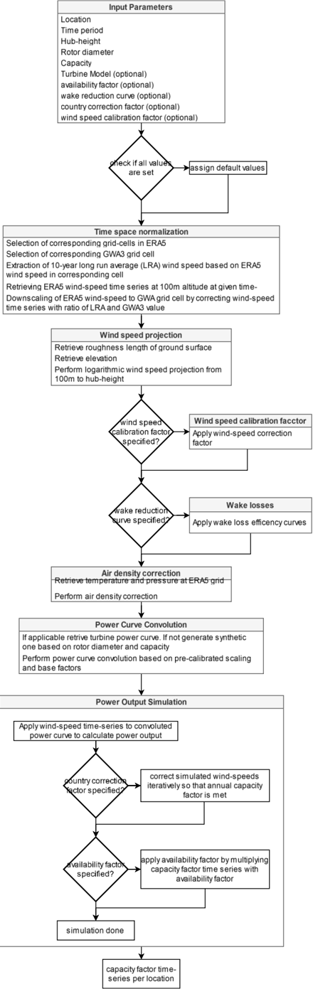
## Flowchart: Wind Power Simulation Process ### Overview The image is a flowchart illustrating the process of wind power simulation. It starts with input parameters, proceeds through time and space normalization, wind speed projection, air density correction, power curve convolution, and finally, power output simulation. Decision points are included to account for optional parameters and corrections. ### Components/Axes The flowchart consists of the following components: 1. **Input Parameters:** A list of required and optional inputs for the simulation. 2. **Process Steps:** Rectangular boxes describing the various stages of the simulation. 3. **Decision Points:** Diamond-shaped boxes representing conditional checks. 4. **Flow Direction:** Arrows indicating the sequence of operations. **Input Parameters:** * Location * Time period * Hub-height * Rotor diameter * Capacity * Turbine Model (optional) * availability factor (optional) * wake reduction curve (optional) * country correction factor (optional) * wind speed calibration factor (optional) ### Detailed Analysis or ### Content Details 1. **Input Parameters:** * The process begins with defining the location, time period, hub-height, rotor diameter, and capacity. * Optional parameters include turbine model, availability factor, wake reduction curve, country correction factor, and wind speed calibration factor. 2. **Initial Check:** * A decision diamond asks "check if all values are set". If not, the process "assign default values". 3. **Time Space Normalization:** * Selection of corresponding grid-cells in ERA5. * Selection of corresponding GWA3 grid cell. * Extraction of 10-year long run average (LRA) wind speed based on ERA5 wind speed in corresponding cell. * Retrieving ERA5 wind-speed time series at 100m altitude at given time. * Downscaling of ERA5 wind-speed to GWA grid cell by correcting wind-speed time series with ratio of LRA and GWA3 value. 4. **Wind Speed Projection:** * Retrieve roughness length of ground surface. * Retrieve elevation. * Perform logarithmic wind speed projection from 100m to hub-height. 5. **Wind Speed Calibration:** * A decision diamond asks "wind speed calibration factor specified?". * If yes, "Apply wind-speed correction factor". 6. **Wake Losses:** * A decision diamond asks "wake reduction curve specified?". * If yes, "Apply wake loss efficiency curves". 7. **Air Density Correction:** * Retrieve temperature and pressure at ERA5 grid. * Perform air density correction. 8. **Power Curve Convolution:** * If applicable, retrieve turbine power curve. If not, generate synthetic one based on rotor diameter and capacity. * Perform power curve convolution based on pre-calibrated scaling and base factors. 9. **Power Output Simulation:** * Apply wind-speed time-series to convoluted power curve to calculate power output. 10. **Country Correction Factor:** * A decision diamond asks "country correction factor specified?". * If yes, "correct simulated wind-speeds iteratively so that annual capacity factor is met". 11. **Availability Factor:** * A decision diamond asks "availability factor specified?". * If yes, "apply availability factor by multiplying capacity factor time series with availability factor". 12. **Final Output:** * "simulation done" * capacity factor time-series per location. ### Key Observations * The flowchart outlines a comprehensive wind power simulation process, incorporating various corrections and adjustments. * Several steps are optional, depending on the availability of specific data or the desired level of accuracy. * The process relies on data from ERA5 and GWA3 datasets. ### Interpretation The flowchart provides a structured approach to simulating wind power generation. It highlights the importance of considering various factors such as location, time period, turbine characteristics, and environmental conditions. The inclusion of optional parameters and correction factors allows for customization and refinement of the simulation, potentially leading to more accurate and reliable results. The iterative correction of simulated wind speeds based on the country correction factor suggests a feedback loop to ensure the annual capacity factor is met, indicating a focus on achieving realistic performance metrics.

\n ## Flowchart: Wind Power Simulation Process ### Overview This image depicts a flowchart outlining the process of wind power simulation, from input parameters to final capacity factor time-series output. The flowchart is structured sequentially, with decision points represented by diamond shapes and process steps by rectangles. Arrows indicate the flow of the process. ### Components/Axes The flowchart consists of the following main sections: 1. **Input Parameters:** A list of parameters used as input for the simulation. 2. **Time space normalization:** Processing of time series data. 3. **Wind speed projection:** Calculation of wind speed at hub height. 4. **Air density correction:** Adjustment for air density. 5. **Power Curve Convolution:** Generation of power output based on wind speed. 6. **Power Output Simulation:** Calculation of capacity factor. 7. **Final Output:** Capacity factor time-series. Decision points involve checks for specified factors (wind speed calibration, wake reduction, country correction, availability). ### Detailed Analysis or Content Details **1. Input Parameters (Top)** * Location * Time period * Hub-height * Rotor diameter * Capacity * Turbine Model (optional) * Availability factor (optional) * Wake reduction curve (optional) * Country correction factor (optional) * Wind speed calibration factor (optional) **2. Check for Default Values:** * If all values are set: Assign default values. **3. Time space normalization:** * Selection of corresponding grid-cells in ERA5 * Selection of corresponding GWA3 grid cell * Extraction of 10-year long run average (LRA) wind speed based on wind speed in corresponding cell * Rescaling ERA5 wind-speed time series at 100m altitude at given time * Downscaling of wind-speed to GWA grid by correcting wind-speed time series with ratio of roughness and GWA height. **4. Wind speed projection:** * Retrieve roughness length of ground surface * Retrieve elevation * Perform logarithmic wind speed projection from 100m to hub-height **5. Wind speed calibration factor:** * If wind speed calibration factor specified?: Apply wind-speed correction factor **6. Wake losses:** * If wake reduction curve specified?: Apply wake loss efficiency curves **7. Air density correction:** * Retrieve temperature and pressure at ERA5 grid * Perform air density correction **8. Power Curve Convolution:** * If applicable retrieve turbine power curve. If not generate synthetic one based on rotor diameter and capacity * Perform power curve convolution based on pre-calibrated scaling and base factors **9. Power Output Simulation:** * Apply wind-speed time-series to convoluted power curve to calculate power output **10. Country corrections:** * If country correction factor specified?: Correct wind-speeds iteratively so total annual capacity factor is met **11. Availability factor:** * If availability factor specified?: Apply availability factor by multiplying capacity factor time series with availability factor **12. Final Output:** * Simulation done * Capacity factor time-series for location ### Key Observations The flowchart highlights a modular approach to wind power simulation. The process is iterative, with decision points allowing for customization based on available data and desired accuracy. The optional parameters suggest that the simulation can be adapted to various scenarios and levels of detail. The iterative correction of wind speeds based on country factors indicates an attempt to account for regional variations and improve the accuracy of the simulation. ### Interpretation This flowchart represents a comprehensive methodology for simulating wind power generation. It demonstrates a clear understanding of the key factors influencing wind turbine performance, including wind speed, air density, wake effects, and turbine characteristics. The inclusion of optional parameters and iterative correction steps suggests a flexible and adaptable simulation framework. The ultimate goal is to generate a reliable capacity factor time-series, which is crucial for assessing the economic viability and grid integration of wind power projects. The process is designed to move from raw input data (location, time period, turbine specs) through a series of increasingly refined calculations to a final output that represents the expected power generation profile. The decision diamonds indicate that the simulation can be tailored to specific conditions, and the iterative correction steps suggest a commitment to accuracy. The flowchart is a valuable tool for engineers and researchers involved in wind energy development and analysis.

## Flowchart: Wind Power Output Simulation Process ### Overview This image is a detailed flowchart illustrating a multi-step computational process for simulating wind power output at a specific location. The process begins with user-defined input parameters, proceeds through data normalization, wind speed projection, and various correction steps, and concludes with a power output simulation to generate a capacity factor time-series. The flow is primarily top-to-bottom, with several decision points that introduce conditional branches. ### Components/Axes The flowchart consists of rectangular process boxes, diamond-shaped decision boxes, and directional arrows indicating the flow of operations. There are no traditional chart axes or legends. The components are organized into a logical sequence. **Top Section: Input Parameters** A large rectangular box lists all required and optional input parameters: * Location * Time period * Hub-height * Rotor diameter * Capacity * Turbine Model (optional) * Availability factor (optional) * Wake reduction curve (optional) * Country correction factor (optional) * Wind speed calibration factor (optional) **Decision Point 1** A diamond box asks: "check if all values are set". * **Yes (implied):** Proceed to "Time space normalization". * **No (implied):** Arrow leads to a process box: "assign default values", which then feeds into "Time space normalization". **Process Block: Time space normalization** A large rectangular box containing a list of sub-steps: 1. Selection of corresponding grid-cells in ERA5 2. Selection of corresponding GWA3 grid cell 3. Extraction of 10-year long run average (LRA) wind speed based on ERA5 wind speed in corresponding cell 4. Retrieving ERA5 wind-speed time series at 100m altitude at given time 5. Downscaling of ERA5 wind-speed to GWA grid cell by correcting wind-speed time series with ratio of LRA and GWA3 value **Process Block: Wind speed projection** A rectangular box containing: * Retrieve roughness length of ground surface * Retrieve elevation * Perform logarithmic wind speed projection from 100m to hub-height **Decision Point 2** A diamond box asks: "wind speed calibration factor specified?". * **Yes:** Arrow leads to a process box: "Wind speed calibration factor / Apply wind-speed correction factor", which then rejoins the main flow. * **No:** Proceed directly to the next decision point. **Decision Point 3** A diamond box asks: "wake reduction curve specified?". * **Yes:** Arrow leads to a process box: "Wake losses / Apply wake loss efficiency curves", which then rejoins the main flow. * **No:** Proceed directly to the next process. **Process Block: Air density correction** A rectangular box containing: * Retrieve temperature and pressure at ERA5 grid * Perform air density correction **Process Block: Power Curve Convolution** A rectangular box containing: * If applicable retrieve turbine power curve. If not generate synthetic one based on rotor diameter and capacity * Perform power curve convolution based on pre-calibrated scaling and base factors **Process Block: Power Output Simulation** A large rectangular box containing the final simulation steps: 1. A process box: "Apply wind-speed time-series to convoluted power curve to calculate power output". 2. **Decision Point 4:** A diamond box asks: "country correction factor specified?". * **Yes:** Arrow leads to a process box: "correct simulated wind-speeds iteratively so that annual capacity factor is met", which then rejoins the main flow. * **No:** Proceed directly to the next decision point. 3. **Decision Point 5:** A diamond box asks: "availability factor specified?". * **Yes:** Arrow leads to a process box: "apply availability factor by multiplying capacity factor time series with availability factor", which then rejoins the main flow. * **No:** Proceed directly to the next step. 4. A final process box: "simulation done". **Final Output** An arrow from the "simulation done" box points to the final output box: "capacity factor time-series per location". ### Detailed Analysis The process is a sequential pipeline with five major conditional branches. The flow is as follows: 1. **Initialization:** Inputs are gathered. Missing optional parameters trigger default assignments. 2. **Data Sourcing & Normalization:** The process sources historical wind data from ERA5 and GWA3 datasets, aligns them spatially and temporally, and downscales the data to the specific location. 3. **Physical Modeling:** Wind speed is projected from the reference height (100m) to the turbine's hub height using surface roughness and elevation data. Optional corrections for site-specific calibration and wake losses can be applied here. 4. **Atmospheric & Turbine Modeling:** Air density is corrected using temperature and pressure data. The turbine's power curve (either retrieved or synthetically generated) is then applied to the corrected wind speed time-series. 5. **Final Adjustments & Output:** The simulated power output undergoes final adjustments. A country-specific correction can be applied iteratively to match a target capacity factor. An availability factor can then be applied to account for downtime. The final product is a time-series of capacity factors for the given location. ### Key Observations * **Modularity and Optionality:** The process is highly modular, with clear separation between data handling, physical correction, and power calculation. Five key parameters are explicitly marked as optional, allowing for simulations of varying complexity and data availability. * **Iterative Correction:** The "country correction factor" step involves an iterative process to meet an annual capacity factor target, indicating a calibration step against known or expected performance. * **Data Dependency:** The process is heavily dependent on external datasets (ERA5, GWA3) for its foundational wind speed data. * **Single Output:** Despite the complex, multi-step process, the final output is a single, specific data product: a capacity factor time-series. ### Interpretation This flowchart represents a sophisticated, physics-based model for estimating the potential energy output of a wind turbine at a specific site. It moves beyond simple average wind speed calculations by incorporating: 1. **Temporal Dynamics:** Using time-series data, not just averages. 2. **Spatial Precision:** Downscaling global/regional data to a specific grid cell. 3. **Physical Realism:** Accounting for hub-height projection, air density, and wake losses. 4. **Operational Realism:** Incorporating availability and country-specific performance corrections. The process is designed to be both **flexible** (through optional parameters) and **rigorous** (through multiple correction stages). The inclusion of iterative correction and synthetic power curve generation suggests it is built to handle real-world scenarios where data may be incomplete or require calibration against known benchmarks. The end goal is to produce a high-fidelity estimate of a wind farm's potential production profile, which is critical for financial modeling, grid integration studies, and resource assessment. The clear, linear flow with defined decision points makes the complex model understandable and likely serves as a blueprint for the software implementation of this simulation tool.

## Flowchart: Wind Power Output Simulation Process ### Overview This flowchart outlines a technical process for simulating wind turbine power output, integrating meteorological data, turbine specifications, and correction factors. The process begins with input parameters, progresses through data normalization, wind speed modeling, and power curve convolution, culminating in a capacity factor time series. ### Components/Axes 1. **Input Parameters** (Top Section): - Mandatory: Location, Time period, Hub-height, Rotor diameter, Capacity - Optional: Turbine Model, Availability factor, Wake reduction curve, Country correction factor, Wind speed calibration factor 2. **Decision Nodes** (Diamond shapes): - "Check if all values are set" - "Wind speed calibration factor specified?" - "Wake reduction curve specified?" - "Country correction factor specified?" - "Availability factor specified?" 3. **Process Steps** (Rectangle shapes): - Time space normalization - Wind speed projection - Air density correction - Power curve convolution - Power output simulation ### Detailed Analysis 1. **Time Space Normalization**: - Aligns ERA5 grid-cell wind-speed data with GWA3 grid-cell data - Uses 10-year long-run average (LRA) for wind-speed extraction - Downsamples ERA5 data to match GWA3 resolution via LRA/GWA3 ratio 2. **Wind Speed Projection**: - Retrieves ground surface roughness and elevation data - Projects wind speed from 100m to hub-height using logarithmic interpolation 3. **Air Density Correction**: - Adjusts for temperature and pressure variations at ERA5 grid locations 4. **Power Curve Convolution**: - Generates turbine power curves using rotor diameter and capacity - Applies pre-calibrated scaling if synthetic curves aren't feasible 5. **Power Output Simulation**: - Applies wind-speed time series to power curves - Iteratively adjusts simulated wind speeds to meet annual capacity factor targets - Incorporates country-specific correction factors and availability factors ### Key Observations - **Mandatory vs Optional Parameters**: 7 mandatory inputs vs 5 optional correction factors - **Data Flow**: Vertical progression from raw meteorological data to final capacity factor output - **Iterative Adjustment**: Final power output simulation includes iterative wind-speed correction - **Geospatial Considerations**: Explicit handling of hub-height adjustments and ground surface roughness ### Interpretation This process demonstrates a comprehensive approach to wind resource assessment and power output prediction. The flowchart emphasizes: 1. **Data Harmonization**: Aligning different resolution datasets (ERA5 vs GWA3) 2. **Physical Adjustments**: Accounting for terrain effects (hub-height projection) and atmospheric conditions (air density) 3. **Operational Realities**: Incorporating turbine-specific parameters and availability factors 4. **Iterative Optimization**: Final simulation adjusts outputs to meet capacity targets The process reveals dependencies between meteorological data quality and final output accuracy, particularly in how wind-speed calibration and wake loss modeling directly impact power curve performance. The optional parameters suggest flexibility for site-specific adjustments while maintaining core simulation integrity.