## Line Chart: Performance Comparison of PIKL and PINN ### Overview The image is a line chart comparing the performance of two methods, PIKL and PINN, against a constant baseline. The chart displays the performance (likely error or loss) on a logarithmic scale as a function of some unspecified variable on a logarithmic scale. The chart includes shaded regions around the lines, representing the uncertainty or variance in the performance of each method. ### Components/Axes * **X-axis:** Logarithmic scale, ranging from 10^1 (10) to 10^5 (100,000). Axis label is not provided. * **Y-axis:** Logarithmic scale, ranging from 10^-4 (0.0001) to 10^-1 (0.1). Axis label is not provided. * **Legend:** Located in the bottom-left corner. * **Constant baseline:** Represented by a black dashed line. * **PIKL:** Represented by a blue line with a light blue shaded region. * **PINN:** Represented by an orange line with a light orange shaded region. ### Detailed Analysis * **Constant Baseline:** A horizontal dashed black line at approximately y = 0.1. * **PIKL (Blue):** * Starts at approximately (10, 0.025) with a shaded region extending from approximately 0.015 to 0.035. * Decreases to approximately (100, 0.01) with a shaded region extending from approximately 0.008 to 0.012. * Decreases sharply to approximately (200, 0.005) with a shaded region extending from approximately 0.004 to 0.006. * Continues to decrease to approximately (10^3, 0.0025) with a shaded region extending from approximately 0.002 to 0.003. * Continues to decrease to approximately (10^4, 0.0007) with a shaded region extending from approximately 0.0005 to 0.0009. * Ends at approximately (10^5, 0.0002) with a shaded region extending from approximately 0.00015 to 0.00025. * **PINN (Orange):** * Starts at approximately (10, 0.015) with a shaded region extending from approximately 0.01 to 0.02. * Decreases to approximately (100, 0.009) with a shaded region extending from approximately 0.007 to 0.011. * Remains relatively constant around 0.008 to 0.01 with a shaded region extending from approximately 0.006 to 0.012. * Ends at approximately (10^5, 0.008) with a shaded region extending from approximately 0.006 to 0.01. ### Key Observations * PIKL consistently outperforms PINN as the x-axis value increases beyond 100. * PIKL shows a significant decrease in value as the x-axis value increases. * PINN's value remains relatively stable after the x-axis value reaches 100. * The shaded regions indicate the uncertainty associated with each method. PIKL's uncertainty decreases as the x-axis value increases, while PINN's uncertainty remains relatively constant. * Both PIKL and PINN start with similar values at the beginning of the chart. ### Interpretation The chart suggests that PIKL is a more effective method than PINN for the task being evaluated, especially as the x-axis value increases. The decreasing value of PIKL indicates that its performance improves with increasing x-axis value, while PINN's stable value suggests that its performance plateaus. The constant baseline provides a reference point, indicating that both methods initially perform worse than the baseline, but PIKL eventually surpasses it. The x-axis is not labeled, so it is difficult to determine what it represents. It could be the number of iterations, the size of the dataset, or some other relevant parameter.

\n ## Line Chart: Error Rate vs. Data Points ### Overview This image presents a line chart comparing the error rates of three methods – PIKL, PINN, and a Constant Baseline – as a function of the number of data points used. The error rate is plotted on a logarithmic scale (y-axis) against the number of data points on a logarithmic scale (x-axis). Each method's performance is represented by a line with a shaded area indicating the uncertainty or variance around the mean. ### Components/Axes * **X-axis:** Labeled "Data Points", with a logarithmic scale ranging from 10¹ to 10⁵. Tick marks are visible at 10¹, 10², 10³, 10⁴, and 10⁵. * **Y-axis:** Labeled "Error Rate", with a logarithmic scale ranging from 10⁻⁴ to 10⁻¹. Tick marks are visible at 10⁻⁴, 10⁻³, 10⁻², and 10⁻¹. * **Legend:** Located in the bottom-left corner. It contains the following entries: * "Constant baseline" – represented by a dashed black line. * "PIKL" – represented by a solid blue line. * "PINN" – represented by a solid orange line. ### Detailed Analysis * **Constant Baseline:** The dashed black line is horizontal and represents a constant error rate of approximately 0.1 (10⁻¹). * **PIKL (Blue Line):** The blue line starts at approximately 0.03 (3 x 10⁻²) at x = 10¹ and slopes downward, decreasing rapidly. At x = 10², the error rate is approximately 0.01 (1 x 10⁻²). The line continues to decrease, reaching approximately 0.0003 (3 x 10⁻⁴) at x = 10⁵. The shaded area around the line indicates a relatively small uncertainty, especially at higher data point values. * **PINN (Orange Line):** The orange line starts at approximately 0.04 (4 x 10⁻²) at x = 10¹ and initially increases slightly, reaching a peak around x = 10². After x = 10², the line plateaus and remains relatively constant, fluctuating between approximately 0.01 (1 x 10⁻²) and 0.02 (2 x 10⁻²). The shaded area around the line is larger than that of PIKL, indicating greater uncertainty. ### Key Observations * PIKL consistently outperforms the Constant Baseline and PINN across all data point values. * PINN's error rate does not decrease significantly with increasing data points, suggesting it may be limited by its method. * The Constant Baseline provides a fixed error rate, serving as a reference point for evaluating the performance of the other methods. * The uncertainty around PINN is significantly higher than that of PIKL, indicating greater variability in its performance. ### Interpretation The chart demonstrates that the PIKL method is significantly more effective at reducing error rates as the number of data points increases compared to PINN. PINN appears to reach a performance plateau, while PIKL continues to improve. The Constant Baseline serves as a benchmark, and both PIKL and PINN outperform it. The smaller uncertainty around PIKL suggests it is a more reliable method. This data suggests that PIKL is a more scalable and robust approach for this particular problem, as its performance improves with more data. PINN, while initially comparable, does not benefit from increased data and exhibits greater variability. The logarithmic scales on both axes emphasize the substantial reduction in error rate achieved by PIKL, particularly as the number of data points grows. The consistent performance of the Constant Baseline highlights the value of the improvements offered by PIKL and PINN.

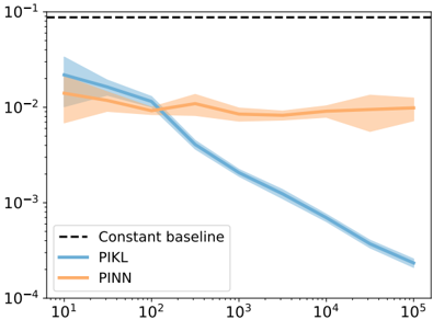
## Line Chart: Performance Comparison of PIKL and PINN Methods ### Overview The image is a line chart plotted on a logarithmic scale (log-log plot) comparing the performance of two methods, PIKL and PINN, against a constant baseline. The chart shows how a performance metric (y-axis) changes as a function of an independent variable (x-axis), likely representing iterations, data size, or a similar parameter. Both methods are shown with shaded regions indicating uncertainty or variance. ### Components/Axes * **Chart Type:** Log-log line chart with shaded confidence/error bands. * **X-Axis:** * **Scale:** Logarithmic (base 10). * **Range:** From `10^1` (10) to `10^5` (100,000). * **Major Tick Labels:** `10^1`, `10^2`, `10^3`, `10^4`, `10^5`. * **Title/Label:** Not explicitly labeled in the image. Represents the independent variable. * **Y-Axis:** * **Scale:** Logarithmic (base 10). * **Range:** From `10^-4` (0.0001) to `10^-1` (0.1). * **Major Tick Labels:** `10^-4`, `10^-3`, `10^-2`, `10^-1`. * **Title/Label:** Not explicitly labeled in the image. Represents a performance metric (e.g., error, loss), where lower values are better. * **Legend:** * **Position:** Bottom-left corner of the plot area. * **Entries:** 1. **Constant baseline:** Represented by a black dashed line (`--`). 2. **PIKL:** Represented by a solid blue line with a light blue shaded band around it. 3. **PINN:** Represented by a solid orange line with a light orange shaded band around it. ### Detailed Analysis **1. Constant Baseline (Black Dashed Line):** * **Trend:** Perfectly horizontal, indicating a constant value. * **Value:** Approximately `y = 10^-1` (0.1) across the entire x-axis range. **2. PIKL (Blue Line & Shaded Band):** * **Trend:** Shows a strong, consistent downward (improving) trend as x increases. The slope is negative and relatively constant on this log-log scale. * **Key Data Points (Approximate):** * At x ≈ `10^1`: y ≈ `2 x 10^-2` (0.02). * At x ≈ `10^2`: y ≈ `10^-2` (0.01). The line crosses below the PINN line near this point. * At x ≈ `10^3`: y ≈ `2 x 10^-3` (0.002). * At x ≈ `10^4`: y ≈ `4 x 10^-4` (0.0004). * At x ≈ `10^5`: y ≈ `2 x 10^-4` (0.0002). * **Uncertainty (Shaded Band):** The band is narrowest at the start (x=10^1) and widens slightly as x increases, but remains relatively tight around the central line. **3. PINN (Orange Line & Shaded Band):** * **Trend:** Shows a relatively flat trend with minor fluctuations. There is no strong upward or downward slope across the range. * **Key Data Points (Approximate):** * At x ≈ `10^1`: y ≈ `1.5 x 10^-2` (0.015). * At x ≈ `10^2`: y ≈ `10^-2` (0.01). The line is crossed by the descending PIKL line. * At x ≈ `10^3`: y ≈ `8 x 10^-3` (0.008). * At x ≈ `10^4`: y ≈ `9 x 10^-3` (0.009). * At x ≈ `10^5`: y ≈ `10^-2` (0.01). * **Uncertainty (Shaded Band):** The band is fairly consistent in width but shows a notable widening at the highest x values (`10^4` to `10^5`), indicating increased variance or uncertainty in the PINN method's performance for large x. ### Key Observations 1. **Performance Crossover:** The PIKL method starts with a slightly higher (worse) value than PINN at low x (`10^1`) but crosses below it around x = `10^2`. For all x > `10^2`, PIKL demonstrates significantly better (lower) performance. 2. **Diverging Trends:** The two methods exhibit fundamentally different behaviors. PIKL improves steadily with increasing x, while PINN's performance stagnates. 3. **Uncertainty Behavior:** The uncertainty for PIKL grows modestly with x. The uncertainty for PINN is stable until very high x, where it increases markedly. 4. **Baseline Comparison:** Both methods consistently perform better (have lower y-values) than the constant baseline of `0.1` across the entire plotted range. ### Interpretation This chart likely compares the convergence or generalization error of two computational methods (PIKL and PINN) as a function of a resource like training iterations, sample size, or model complexity (x-axis). * **PIKL demonstrates superior scalability.** Its consistent downward trend on the log-log plot suggests a power-law relationship, where performance improves predictably as more resources (x) are allocated. This is a highly desirable property for an algorithm. * **PINN shows limited benefit from increased resources.** Its flat trend indicates that beyond a certain point (x ≈ `10^2`), allocating more resources does not lead to meaningful improvement. The widening uncertainty at high x further suggests potential instability or sensitivity in the method under those conditions. * **The "Constant baseline"** serves as a reference point, showing that both advanced methods are effective compared to a naive or fixed approach. * **Practical Implication:** If the goal is to achieve the lowest possible error and resources (x) are available, PIKL is the clear choice. If resources are severely limited (x < `10^2`), PINN might offer a slight initial advantage, but this advantage is quickly overtaken by PIKL. The investigation would focus on understanding the algorithmic reasons why PIKL scales effectively while PINN plateaus.

## Line Graph: Performance Comparison of Baselines and Models ### Overview The image is a logarithmic line graph comparing three performance metrics across a range of input values (x-axis: 10¹ to 10⁵). The y-axis represents a normalized metric (10⁻¹ to 10⁻⁴). Three lines are plotted: a constant baseline (dashed black), PIKL baseline (solid blue), and PINN (solid orange), with shaded regions indicating uncertainty. ### Components/Axes - **Y-axis**: Logarithmic scale labeled 10⁻¹ (top) to 10⁻⁴ (bottom), with gridlines at 10⁻² and 10⁻³. - **X-axis**: Logarithmic scale labeled 10¹ (left) to 10⁵ (right), with gridlines at 10², 10³, 10⁴. - **Legend**: Positioned at the bottom-left corner, with three entries: - Dashed black: "Constant baseline" - Solid blue: "PIKL baseline" - Solid orange: "PINN" - **Shaded Regions**: Light blue (PIKL) and light orange (PINN) bands around the lines, representing uncertainty. ### Detailed Analysis 1. **Constant Baseline (Dashed Black)**: - Horizontal line at y = 10⁻² (0.01) across all x-values. - No variation or uncertainty shading. 2. **PIKL Baseline (Solid Blue)**: - Starts at ~10⁻¹.⁵ (≈3×10⁻²) at x = 10¹. - Declines steeply, crossing the PINN line near x = 10². - Continues declining to ~10⁻³.⁵ (≈3×10⁻⁴) at x = 10⁵. - Shaded region widens at lower x-values, narrowing as x increases. 3. **PINN (Solid Orange)**: - Starts at ~10⁻².⁵ (≈3×10⁻³) at x = 10¹. - Rises slightly to ~10⁻² at x = 10², then plateaus. - Remains above the PIKL line after x = 10². - Shaded region is narrower than PIKL’s, indicating lower uncertainty. ### Key Observations - **Crossover Point**: PIKL and PINN intersect near x = 10², after which PINN outperforms PIKL. - **Uncertainty**: PIKL’s uncertainty is higher at lower x-values (10¹–10²) but decreases as x increases. - **Baseline Stability**: The constant baseline remains unchanged, serving as a reference for relative performance. ### Interpretation The graph demonstrates that PINN outperforms the PIKL baseline for x > 10², suggesting improved performance or stability at higher input scales. The constant baseline (10⁻²) may represent a theoretical or empirical threshold. The narrowing uncertainty bands for both models at higher x-values imply increased confidence in their predictions as input magnitude grows. This could indicate that PINN is better suited for high-scale applications, while PIKL’s variability at lower scales might limit its reliability. The constant baseline’s fixed value highlights a potential target or benchmark for both models.