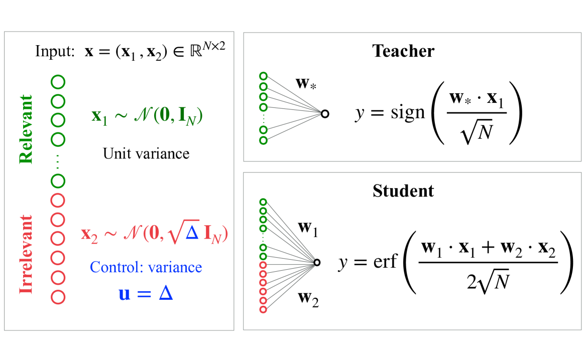
## Diagram: Teacher-Student Model ### Overview The image presents a diagram illustrating a teacher-student model, likely within a machine learning or statistical learning context. It depicts two parallel processing pathways – one for a "Teacher" and one for a "Student" – both receiving input **x** which is a vector composed of **x₁** and **x₂**. The diagram details the mathematical operations performed by each pathway and highlights the differing characteristics of the input components. ### Components/Axes The diagram is structured into three main sections: Input, Teacher, and Student. * **Input:** Defines the input vector **x** as belonging to ℝ^(N×2). It specifies that **x₁** is drawn from a normal distribution with mean **0** and identity matrix **I_N** (unit variance), and **x₂** is drawn from a normal distribution with mean **0** and √Δ**I_N** (control variance). * **Teacher:** Shows a network with weights **w*** and an output **y** calculated using the sign function applied to the dot product of **w*** and **x₁**, scaled by 1/√N. * **Student:** Shows a network with weights **w₁** and **w₂** and an output **y** calculated using the error function (erf) applied to the dot product of **w₁** and **x₁** plus the dot product of **w₂** and **x₂**, scaled by 2/√N. * **Legend:** A vertical legend on the left side distinguishes between "Relevant" (green circles) and "Irrelevant" (black circles) input components. * **Variables:** **u = Δ** is defined as a control variance parameter. ### Detailed Analysis or Content Details The diagram details the following mathematical relationships: * **Input:** **x** = ( **x₁**, **x₂**) ∈ ℝ^(N×2) * **x₁** ~ *N*(**0**, **I_N**) – **x₁** follows a normal distribution with mean vector **0** and covariance matrix equal to the identity matrix **I_N**. * **x₂** ~ *N*(**0**, √Δ**I_N**) – **x₂** follows a normal distribution with mean vector **0** and covariance matrix equal to √Δ times the identity matrix **I_N**. * **Teacher Output:** y = sign( (**w*** ⋅ **x₁**) / √N ) * **Student Output:** y = erf( (**w₁** ⋅ **x₁** + **w₂** ⋅ **x₂**) / (2√N) ) The legend indicates that **x₁** is considered "Relevant" (represented by green circles) while **x₂** is considered "Irrelevant" (represented by black circles). The diagram visually represents the flow of information through each network. The Teacher network receives only the relevant input **x₁**, while the Student network receives both **x₁** and **x₂**. ### Key Observations * The Teacher network uses a sign function, resulting in a binary output. * The Student network uses the error function (erf), resulting in a continuous output between -1 and 1. * The scaling factor (1/√N for the Teacher and 2/√N for the Student) suggests a normalization or variance control mechanism. * The control variance parameter Δ in **x₂** allows for manipulation of the irrelevant input's influence. * The diagram highlights a clear distinction between the inputs used by the Teacher and the Student, suggesting a learning scenario where the Student attempts to mimic the Teacher's behavior despite having access to irrelevant information. ### Interpretation This diagram illustrates a scenario where a Student network is trained to replicate the behavior of a Teacher network. The Teacher operates on a simplified input space consisting only of "relevant" features (**x₁**), while the Student is exposed to both relevant and "irrelevant" features (**x₁** and **x₂**). The use of different activation functions (sign vs. erf) and scaling factors suggests that the Student network may need to learn to filter out the irrelevant information and approximate the Teacher's output. The parameter Δ controlling the variance of **x₂** is crucial. A larger Δ would mean the irrelevant input has a larger impact, making the Student's task more challenging. The diagram suggests a study of robustness to irrelevant features or a method for learning feature selection. The use of the error function in the Student network implies a probabilistic interpretation of the output, while the sign function in the Teacher network suggests a deterministic decision boundary. This setup could be used to investigate how a student can learn to ignore irrelevant information and focus on the essential features for accurate prediction.