## Diagram: Input Processing and Model Comparison
### Overview
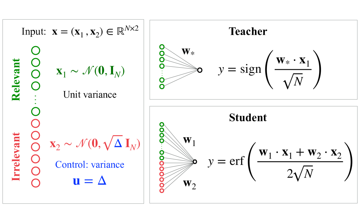
The image compares two models ("Teacher" and "Student") processing input vectors with relevant and irrelevant components. The left side defines input distributions, while the right side illustrates model architectures and output calculations.
### Components/Axes
#### Left Panel (Input Definitions):
- **Labels**:
- "Relevant" (green circles): `x₁ ~ N(0, I_N)` (unit variance)
- "Irrelevant" (red circles): `x₂ ~ N(0, √Δ I_N)` (controlled variance, `u = Δ`)
- **Input**: `x = (x₁, x₂) ∈ ℝ^(N×2)`
- **Legend**:
- Green circles = Relevant features
- Red circles = Irrelevant features
#### Right Panel (Model Architectures):
- **Teacher**:
- Single weight vector `w*`
- Output: `y = sign(w* · x₁ / √N)`
- **Student**:
- Two weight vectors `w₁` (green) and `w₂` (red)
- Output: `y = erf((w₁ · x₁ + w₂ · x₂) / (2√N))`
### Detailed Analysis
#### Input Distributions:
- **Relevant (`x₁`)**:
- Mean = 0, Covariance = Identity matrix `I_N` (unit variance).
- Visualized as green circles with uniform spacing.
- **Irrelevant (`x₂`)**:
- Mean = 0, Covariance = `√Δ I_N` (variance scaled by `Δ`).
- Visualized as red circles with spacing proportional to `√Δ`.
#### Model Equations:
- **Teacher**:
- Simplified binary classifier using `sign()` function.
- Normalization: `w* · x₁ / √N` (reduces variance of input).
- **Student**:
- Combines `w₁` (green) and `w₂` (red) with equal weighting.
- Uses `erf()` (error function) for non-linear transformation.
- Normalization: `2√N` in denominator (doubles scaling compared to Teacher).
#### Spatial Relationships:
- **Left Panel**:
- Relevant (green) and irrelevant (red) inputs are vertically stacked.
- Variance control (`u = Δ`) is explicitly labeled in blue.
- **Right Panel**:
- Teacher and Student models are horizontally separated.
- Weights (`w*`, `w₁`, `w₂`) are connected to inputs via lines.
### Key Observations
1. **Variance Control**:
- Irrelevant features (`x₂`) have variance `√Δ`, adjustable via `Δ`.
- Relevant features (`x₁`) maintain fixed unit variance.
2. **Model Complexity**:
- Teacher uses a single weight and linear thresholding (`sign()`).
- Student uses two weights and a non-linear `erf()` function.
3. **Color Consistency**:
- Green weights (`w₁`) align with relevant inputs (`x₁`).
- Red weights (`w₂`) align with irrelevant inputs (`x₂`).
### Interpretation
The diagram illustrates a **feature selection and model adaptation** scenario:
- The **Teacher** focuses solely on relevant features (`x₁`), discarding irrelevant ones (`x₂`).
- The **Student** attempts to learn from both relevant and irrelevant features, using a more complex non-linear model (`erf()`).
- The variance control (`Δ`) suggests a trade-off: increasing `Δ` amplifies irrelevant feature noise, potentially degrading performance unless the Student model can effectively suppress it.
- The use of `erf()` in the Student model implies an attempt to model probabilistic or smooth decision boundaries, contrasting with the Teacher’s hard thresholding.
This setup likely explores how models handle noisy or redundant inputs and whether students can generalize better by leveraging additional features, even irrelevant ones, through adaptive weighting.