## Diagram: Teacher-Student Neural Network Architecture with Dropout and Rescaling
### Overview
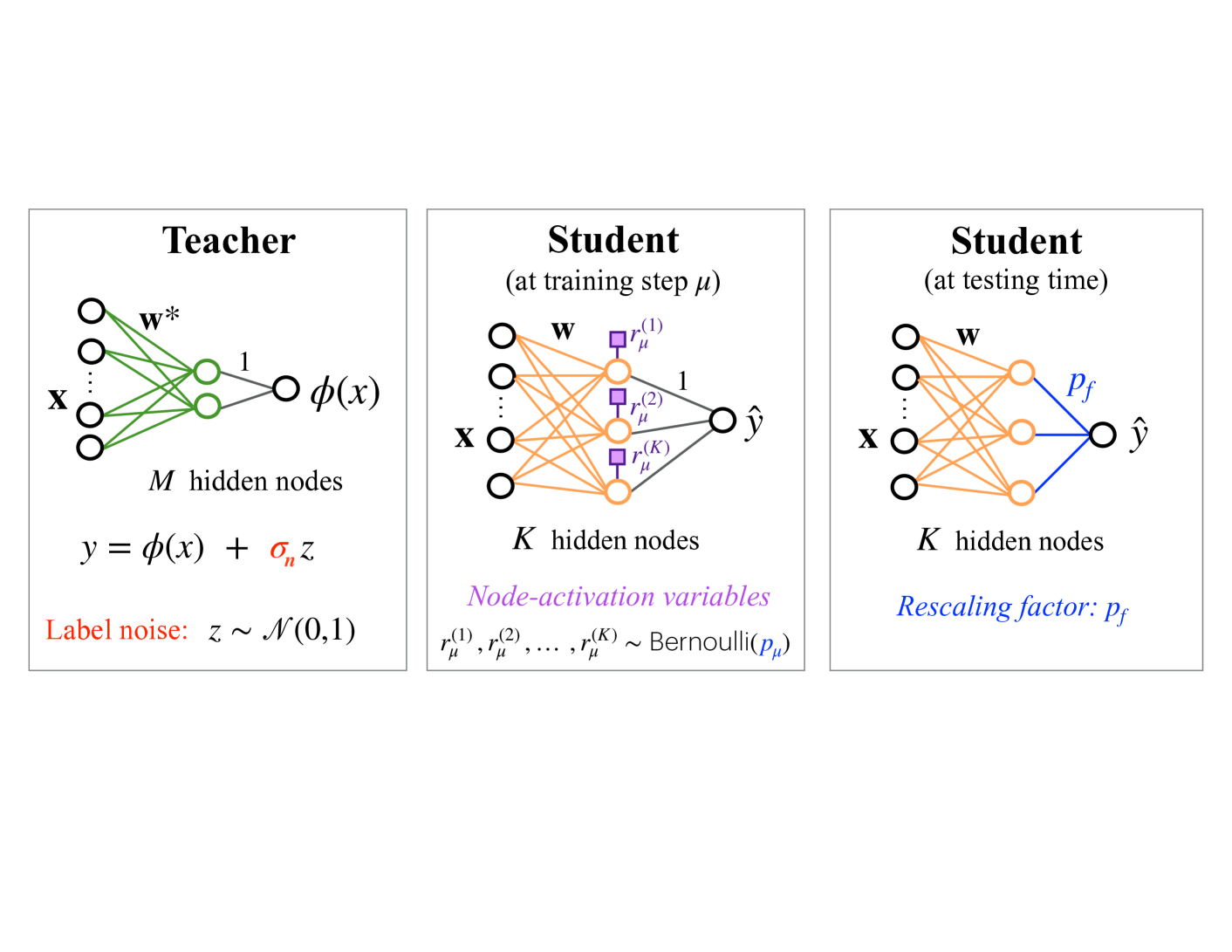
The image is a technical diagram illustrating a teacher-student learning framework for neural networks, specifically depicting a process involving label noise, dropout during training, and a rescaling factor during testing. It consists of three distinct panels arranged horizontally, each showing a feedforward neural network architecture with associated mathematical notation and explanatory text.
### Components/Axes
The diagram is divided into three rectangular panels, each with a title and containing a neural network schematic.
**Panel 1 (Left): "Teacher"**
* **Network Structure:** A neural network with an input layer (labeled **x**), a single hidden layer with **M hidden nodes**, and a single output node.
* **Connections:** Green lines connect the input nodes to the hidden nodes. The connections from the hidden layer to the output node are labeled with the number **1**.
* **Weights:** The connections from input to hidden are labeled **w***.
* **Output:** The output of the hidden layer transformation is denoted as **φ(x)**.
* **Equation:** Below the network: `y = φ(x) + σ_n z`
* **Label Noise Definition:** Text in red: "Label noise: z ~ N(0,1)" (indicating z is drawn from a standard normal distribution).
**Panel 2 (Center): "Student (at training step μ)"**
* **Network Structure:** A neural network with an input layer (labeled **x**), a single hidden layer with **K hidden nodes**, and a single output node producing **ŷ**.
* **Connections:** Orange lines connect the input nodes to the hidden nodes. The connections from the hidden layer to the output node are labeled with the number **1**.
* **Weights:** The connections from input to hidden are labeled **w**.
* **Node-Activation Variables:** Purple squares are placed on the connections from the hidden layer to the output. They are labeled **r_μ^(1)**, **r_μ^(2)**, and **r_μ^(K)**.
* **Text (Purple):** "Node-activation variables"
* **Equation:** `r_μ^(1), r_μ^(2), ..., r_μ^(K) ~ Bernoulli(p_μ)` (indicating each activation variable is an independent Bernoulli random variable with probability p_μ).
**Panel 3 (Right): "Student (at testing time)"**
* **Network Structure:** Identical to the Student at training: input **x**, **K hidden nodes**, output **ŷ**.
* **Connections:** Orange lines connect input to hidden. The connections from the hidden layer to the output are colored **blue**.
* **Weights:** The connections from input to hidden are labeled **w**.
* **Rescaling Factor:** The blue output connections are collectively labeled **p_f**.
* **Text (Blue):** "Rescaling factor: p_f"
### Detailed Analysis
* **Teacher Network:** Represents a fixed, pre-trained model. It generates the target signal `φ(x)` but the observed training label `y` is corrupted by additive Gaussian noise with standard deviation `σ_n`.
* **Student Network (Training):** The student network learns from the noisy teacher. A key feature is the application of dropout to the hidden layer's output during training. Each of the K hidden nodes' contributions to the output is independently multiplied by a Bernoulli random variable `r_μ^(k)` (which is 1 with probability `p_μ` and 0 otherwise). This simulates randomly "dropping out" nodes.
* **Student Network (Testing):** At inference time, all K hidden nodes are active. To compensate for the fact that only a fraction `p_μ` of nodes were active on average during training, the combined output from the hidden layer is scaled by a factor `p_f`. The diagram implies `p_f` is related to `p_μ` (commonly `p_f = p_μ` in standard dropout implementation).
### Key Observations
1. **Architectural Consistency:** The student network has the same structure (K hidden nodes) in both training and testing phases, but the processing of the hidden layer's output differs.
2. **Color Coding:** Colors are used functionally: Green for the teacher's weights, orange for the student's weights, purple for the stochastic training-time dropout variables, and blue for the deterministic testing-time rescaling factor.
3. **Parameter Notation:** The teacher uses `w*` (optimal/fixed weights), while the student uses `w` (learned weights). The teacher has `M` hidden nodes, while the student has `K` hidden nodes (where K may or may not equal M).
4. **Noise Model:** Label noise is explicitly modeled as additive Gaussian noise `N(0,1)` scaled by `σ_n`.
### Interpretation
This diagram visually explains the mechanics of **knowledge distillation** combined with **dropout regularization**. The teacher network provides a "soft target" `φ(x)`, which is a richer training signal than hard labels but is further corrupted by noise. The student network learns to mimic this signal.
The core insight is the depiction of dropout's train-test discrepancy. During training (center panel), the student's learning is stochastic due to the Bernoulli masking (`r_μ`), which acts as a regularizer preventing co-adaptation of nodes. At test time (right panel), the network becomes deterministic, but its output must be rescaled by `p_f` to account for the fact that all nodes are now active, ensuring the expected magnitude of the output matches what was seen during training. The diagram effectively isolates and contrasts these two operational modes of the same student network. The presence of the teacher and label noise suggests this framework might be used for learning from noisy data or for model compression where a large teacher guides a smaller student.