## [Diagram/Graph Pair]: Network Graphs and Adjacency Matrices
### Overview
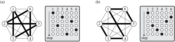
The image displays two side-by-side panels, labeled (a) and (b). Each panel contains a pair of related diagrams: a **network graph** on the left and a corresponding **adjacency matrix** (or step matrix) on the right. The diagrams appear to represent connectivity or relationships between six numbered nodes (1 through 6) in two different states or configurations.
### Components/Axes
**Panel (a):**
* **Left - Network Graph:**
* **Nodes:** Six circles numbered 1, 2, 3, 4, 5, 6 arranged in a hexagonal pattern.
* **Edges:** Lines connecting the nodes. The lines have two distinct thicknesses: **thick** and **thin**.
* **Spatial Layout:** Node 1 is at the top. Nodes 2 and 6 are at the upper left and right. Nodes 3 and 5 are at the lower left and right. Node 4 is at the bottom.
* **Right - Adjacency Matrix:**
* **Structure:** A 6x6 grid of circles.
* **Axes Labels:**
* **Top (Columns):** Numbers 1, 2, 3, 4, 5, 6.
* **Left (Rows):** The word "step" written vertically, with an arrow pointing downward. This implies the rows represent sequential steps or time.
* **Data Points:** Circles within the grid are either **filled (black)** or **empty (white outline)**. A filled circle indicates an active connection or relationship between the column node and the row step.
**Panel (b):**
* **Left - Network Graph:**
* **Nodes:** Same hexagonal arrangement of nodes 1-6.
* **Edges:** Lines connecting nodes, again with **thick** and **thin** lines. The pattern of thick lines is different from panel (a).
* **Right - Adjacency Matrix:**
* **Structure:** Identical 6x6 grid layout as in (a).
* **Axes Labels:** Identical to (a): Column numbers 1-6, and a vertical "step" label with a downward arrow on the left.
* **Data Points:** A different pattern of filled (black) and empty (white) circles compared to panel (a).
### Detailed Analysis
**Panel (a) Analysis:**
* **Graph Connectivity (Thick Lines):** The thick edges form a specific subgraph. They connect:
* Node 1 to Node 3
* Node 1 to Node 4
* Node 1 to Node 5
* Node 2 to Node 4
* Node 2 to Node 5
* Node 3 to Node 6
* Node 4 to Node 6
* Node 5 to Node 6
* **Matrix Data (Filled Circles):** The filled circles in the matrix correspond to the following (Row "step" / Column Node):
* Step 1: Node 1
* Step 2: Node 3
* Step 3: Node 2
* Step 4: Node 5
* Step 5: Node 4
* Step 6: Node 6
* **Mapping:** The matrix does not directly show the graph's adjacency. Instead, it seems to show a **sequence or activation order** of the nodes over 6 steps. The pattern of filled circles is a single filled circle per row, moving down the steps.
**Panel (b) Analysis:**
* **Graph Connectivity (Thick Lines):** The thick edges form a different subgraph. They connect:
* Node 1 to Node 6
* Node 2 to Node 5
* Node 3 to Node 4
* Node 3 to Node 6
* Node 4 to Node 5
* **Matrix Data (Filled Circles):** The filled circles show a different pattern:
* Step 1: Node 1
* Step 2: Node 2
* Step 3: Node 3
* Step 4: Node 4
* Step 5: Node 5
* Step 6: Node 6
* **Mapping:** Similar to (a), this matrix shows a node activation sequence. The sequence here is a simple diagonal: Node 1 at step 1, Node 2 at step 2, etc., through Node 6 at step 6.
### Key Observations
1. **Different Graph Topologies:** The two graphs have distinct sets of "thick" edges, indicating two different network structures or states.
2. **Different Activation Sequences:** The matrices show two different temporal patterns. Panel (a) shows a non-sequential, seemingly random order of node activation (1, 3, 2, 5, 4, 6). Panel (b) shows a perfectly sequential order (1, 2, 3, 4, 5, 6).
3. **Matrix Interpretation:** The matrices are not standard adjacency matrices (which would show all connections at once). The "step" axis and single filled circle per row strongly suggest they represent a **time series** or **process flow** where one node is active or selected at each discrete step.
4. **Potential Relationship:** The thick edges in the graph might represent the **available or strong connections** at the start, while the matrix shows the **actual path or activation sequence** taken through the network over time.
### Interpretation
This figure likely illustrates a concept in **network science, graph theory, or dynamic systems**. It contrasts two scenarios:
* **Scenario (a):** A network with a complex, highly interconnected structure (many thick edges) is traversed in a non-intuitive, non-sequential order. The path (1→3→2→5→4→6) jumps across the network, possibly following a rule like "activate the node with the strongest connection to the currently active node" or representing a stochastic process.
* **Scenario (b):** A network with a simpler, more linear or ring-like structure of thick edges (1-6, 2-5, 3-4, plus 3-6 and 4-5) is traversed in a perfectly sequential order (1→2→3→4→5→6). This suggests a more predictable, perhaps rule-based or spatially-ordered process.
The core message is the relationship between **network structure** (the graph) and **dynamic behavior** (the sequence in the matrix). The same set of nodes can exhibit vastly different temporal patterns depending on the underlying connectivity. The thick lines may represent "highways" or preferred pathways that constrain or guide the sequential activation shown in the matrices. The figure demonstrates how structural properties of a network influence its functional dynamics over time.