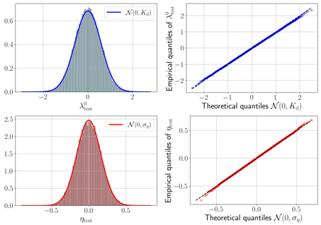
## Chart Type: Distribution and Quantile-Quantile (Q-Q) Plots ### Overview The image presents four plots arranged in a 2x2 grid. The top-left and bottom-left plots are histograms overlaid with normal distribution curves. The top-right and bottom-right plots are quantile-quantile (Q-Q) plots, comparing empirical quantiles against theoretical quantiles from normal distributions. ### Components/Axes **Top-Left Plot:** * **Type:** Histogram with overlaid normal distribution curve * **X-axis:** λ⁰test, ranging from approximately -2 to 2. * **Y-axis:** Implicitly represents frequency or density, ranging from 0.0 to 0.6. * **Curve:** Blue curve labeled "N(0, Kd)", representing a normal distribution with mean 0 and standard deviation Kd. * **Bars:** Gray bars representing the histogram of the data. **Top-Right Plot:** * **Type:** Quantile-Quantile (Q-Q) plot * **X-axis:** Theoretical quantiles N(0, Kd), ranging from approximately -2 to 2. * **Y-axis:** Empirical quantiles of λ⁰test, ranging from approximately -2 to 2. * **Data Points:** Blue dots representing the quantiles. **Bottom-Left Plot:** * **Type:** Histogram with overlaid normal distribution curve * **X-axis:** ηtest, ranging from approximately -0.5 to 0.5. * **Y-axis:** Implicitly represents frequency or density, ranging from 0.0 to 2.5. * **Curve:** Red curve labeled "N(0, ση)", representing a normal distribution with mean 0 and standard deviation ση. * **Bars:** Red bars representing the histogram of the data. **Bottom-Right Plot:** * **Type:** Quantile-Quantile (Q-Q) plot * **X-axis:** Theoretical quantiles N(0, ση), ranging from approximately -0.5 to 0.5. * **Y-axis:** Empirical quantiles of ηtest, ranging from approximately -0.5 to 0.5. * **Data Points:** Red dots representing the quantiles. * **Reference Line:** Dashed black line representing y=x. ### Detailed Analysis **Top-Left Plot (λ⁰test Distribution):** * The histogram shows a distribution centered around 0. * The blue curve "N(0, Kd)" closely fits the histogram, suggesting the data is approximately normally distributed with a mean of 0. * The peak of the distribution is around 0.6 on the y-axis. **Top-Right Plot (λ⁰test Q-Q Plot):** * The blue dots closely follow a straight line, indicating that the empirical distribution of λ⁰test is close to a normal distribution. * There is a slight deviation from the line at the extreme tails. **Bottom-Left Plot (ηtest Distribution):** * The histogram shows a distribution centered around 0. * The red curve "N(0, ση)" closely fits the histogram, suggesting the data is approximately normally distributed with a mean of 0. * The peak of the distribution is around 2.5 on the y-axis. **Bottom-Right Plot (ηtest Q-Q Plot):** * The red dots closely follow the dashed black line, indicating that the empirical distribution of ηtest is close to a normal distribution. * There is a slight deviation from the line at the extreme tails. ### Key Observations * Both λ⁰test and ηtest appear to be approximately normally distributed with a mean of 0. * The Q-Q plots confirm the normality, with minor deviations at the tails. * The distribution of ηtest has a higher peak (2.5) than the distribution of λ⁰test (0.6), indicating a smaller standard deviation. ### Interpretation The plots suggest that both λ⁰test and ηtest are well-modeled by normal distributions with a mean of 0. The Q-Q plots provide a visual assessment of how well the empirical distributions match the theoretical normal distributions. The close alignment of the points with the straight line in the Q-Q plots indicates a good fit, with only slight deviations at the extreme quantiles. This suggests that the assumption of normality is reasonable for these datasets. The difference in peak heights between the two distributions indicates that ηtest has a smaller standard deviation than λ⁰test.

## Chart Type: Statistical Distribution and Q-Q Plots ### Overview The image consists of a 2x2 grid of statistical plots used to analyze the distribution of two variables: $\lambda^0_{\text{test}}$ (top row) and $\eta_{\text{test}}$ (bottom row). Each row contains a histogram with an overlaid probability density function (PDF) on the left and a corresponding Quantile-Quantile (Q-Q) plot on the right. The plots serve to verify if the empirical data follows a specific theoretical normal distribution. --- ### Components/Axes #### Top Row: Analysis of $\lambda^0_{\text{test}}$ * **Top-Left Plot (Histogram & PDF):** * **X-axis:** Labelled $\lambda^0_{\text{test}}$. Range: $\approx [-3.0, 3.0]$. Major ticks at $-2, 0, 2$. * **Y-axis:** Probability density. Range: $[0.0, 0.7]$. Major ticks at $0.0, 0.2, 0.4, 0.6$. * **Legend (Top-Right):** Blue solid line labeled $\mathcal{N}(0, K_d)$. * **Top-Right Plot (Q-Q Plot):** * **X-axis:** Labelled "Theoretical quantiles $\mathcal{N}(0, K_d)$". Range: $\approx [-2.5, 2.5]$. * **Y-axis:** Labelled "Empirical quantiles of $\lambda^0_{\text{test}}$". Range: $\approx [-2.5, 2.5]$. * **Legend:** None (implicit reference line). #### Bottom Row: Analysis of $\eta_{\text{test}}$ * **Bottom-Left Plot (Histogram & PDF):** * **X-axis:** Labelled $\eta_{\text{test}}$. Range: $\approx [-0.8, 0.8]$. Major ticks at $-0.5, 0.0, 0.5$. * **Y-axis:** Probability density. Range: $[0.0, 2.5]$. Major ticks at $0.0, 0.5, 1.0, 1.5, 2.0, 2.5$. * **Legend (Top-Right):** Red solid line labeled $\mathcal{N}(0, \sigma_\eta)$. * **Bottom-Right Plot (Q-Q Plot):** * **X-axis:** Labelled "Theoretical quantiles $\mathcal{N}(0, \sigma_\eta)$". Range: $\approx [-0.8, 0.8]$. * **Y-axis:** Labelled "Empirical quantiles of $\eta_{\text{test}}$". Range: $\approx [-0.8, 0.8]$. * **Legend:** None (implicit reference line). --- ### Content Details #### 1. Distribution of $\lambda^0_{\text{test}}$ (Top Row) * **Histogram/PDF Trend:** The data shows a symmetric, bell-shaped distribution centered exactly at $0$. The blue PDF curve $\mathcal{N}(0, K_d)$ tracks the heights of the grey histogram bars very closely. The peak density is approximately $0.7 \pm 0.02$. * **Q-Q Plot Trend:** The data points (blue circles) form a nearly perfect straight line sloping upward at a 45-degree angle, coinciding with the dashed black reference line ($y=x$). This indicates a strong match between the empirical data and the theoretical normal distribution. #### 2. Distribution of $\eta_{\text{test}}$ (Bottom Row) * **Histogram/PDF Trend:** Similar to the top row, this distribution is symmetric and centered at $0$. However, it is much narrower and taller. The red PDF curve $\mathcal{N}(0, \sigma_\eta)$ fits the red-tinted histogram bars well. The peak density is significantly higher, reaching approximately $2.45 \pm 0.05$. * **Q-Q Plot Trend:** The data points (red circles) follow the dashed black reference line closely. There is a very slight "tailing off" or jitter at the extreme ends (near $-0.7$ and $0.7$), but the overall trend is strictly linear along $y=x$. --- ### Key Observations * **Scale Difference:** The variable $\lambda^0_{\text{test}}$ has a much larger variance/spread (roughly 3 units from the mean) compared to $\eta_{\text{test}}$ (roughly 0.7 units from the mean). * **Normality:** Both variables exhibit characteristics of a normal distribution with a mean of zero. * **Fit Quality:** The Q-Q plots confirm that the theoretical models ($\mathcal{N}(0, K_d)$ and $\mathcal{N}(0, \sigma_\eta)$) are excellent representations of the observed test data. --- ### Interpretation The data demonstrates a successful validation of statistical assumptions. In many technical or scientific contexts (such as signal processing or machine learning), it is crucial to prove that residuals or test statistics follow a predicted normal distribution. * **$\lambda^0_{\text{test}}$ vs $\eta_{\text{test}}$:** The difference in the Y-axis scales of the histograms (0.7 vs 2.5) suggests that $\eta_{\text{test}}$ is a "tighter" or more precise measurement than $\lambda^0_{\text{test}}$, assuming they measure similar phenomena. * **Statistical Significance:** The tight alignment in the Q-Q plots suggests that there are no significant outliers or heavy tails in the data that would violate the normality assumption. This justifies the use of Gaussian-based statistical tests or models for these specific variables. * **Peircean Investigation:** The presence of these plots usually implies a "Goodness of Fit" step in a larger experiment. The researcher is showing the reader that the underlying math (the normal distribution) is not just a guess, but a verified reality of the dataset.

\n ## Statistical Plots: Normal Distribution and Quantile-Quantile Plots ### Overview The image presents four statistical plots. The top two plots relate to a normal distribution N(0, K_σ), while the bottom two relate to a normal distribution N(0, σ₀). The left-hand plots are histograms showing the probability density function, and the right-hand plots are quantile-quantile (Q-Q) plots comparing the empirical quantiles of a test statistic to the theoretical quantiles of the corresponding normal distribution. ### Components/Axes * **Top Left (Histogram):** * X-axis: λ_test (ranging approximately from -2 to 2) * Y-axis: Probability Density (ranging approximately from 0 to 0.6) * Curve Label: N(0, K_σ) - Blue * **Top Right (Q-Q Plot):** * X-axis: Theoretical quantiles N(0, K_σ) (ranging approximately from -2 to 2) * Y-axis: Empirical quantiles of λ_test (ranging approximately from -2 to 2) * **Bottom Left (Histogram):** * X-axis: θ_test (ranging approximately from -0.5 to 0.5) * Y-axis: Probability Density (ranging approximately from 0 to 2.5) * Curve Label: N(0, σ₀) - Red * **Bottom Right (Q-Q Plot):** * X-axis: Theoretical quantiles N(0, σ₀) (ranging approximately from -0.5 to 0.5) * Y-axis: Empirical quantiles of θ_test (ranging approximately from -0.5 to 0.5) ### Detailed Analysis or Content Details * **Top Left Histogram:** The blue curve represents a normal distribution N(0, K_σ). The distribution is centered around 0, with a spread determined by K_σ. The peak of the distribution is approximately at 0.6. * **Top Right Q-Q Plot:** The blue points form a nearly straight line. This indicates that the empirical quantiles of λ_test closely follow the theoretical quantiles of N(0, K_σ), suggesting that λ_test is approximately normally distributed. There is a slight curvature, indicating a possible deviation from perfect normality. * **Bottom Left Histogram:** The red curve represents a normal distribution N(0, σ₀). The distribution is centered around 0, with a spread determined by σ₀. The peak of the distribution is approximately at 2.5. * **Bottom Right Q-Q Plot:** The red points also form a nearly straight line. This indicates that the empirical quantiles of θ_test closely follow the theoretical quantiles of N(0, σ₀), suggesting that θ_test is approximately normally distributed. There is a slight curvature, indicating a possible deviation from perfect normality. ### Key Observations * Both λ_test and θ_test appear to be approximately normally distributed, as evidenced by the Q-Q plots. * The distributions N(0, K_σ) and N(0, σ₀) have different spreads, as indicated by the histograms. N(0, σ₀) has a wider spread than N(0, K_σ). * The Q-Q plots show slight deviations from a perfectly straight line, suggesting that the normality assumption may not be perfectly met for either λ_test or θ_test. ### Interpretation The image demonstrates the assessment of normality for two test statistics, λ_test and θ_test. The histograms visualize the probability density functions of these statistics, while the Q-Q plots provide a more formal assessment of normality by comparing empirical and theoretical quantiles. The near-linear patterns in the Q-Q plots suggest that both statistics are approximately normally distributed, which is a common assumption in many statistical tests. The differences in the spreads of the distributions suggest that K_σ and σ₀ are different parameters, likely representing different scales or variances. The slight curvature in the Q-Q plots indicates that the normality assumption should be considered cautiously, and further investigation may be warranted to assess the extent of any deviations from normality. The image is a standard diagnostic tool used in statistical modeling to verify model assumptions.

## Statistical Distribution Analysis: Histograms and Q-Q Plots ### Overview The image is a 2x2 grid of four statistical plots. The top row analyzes a variable labeled \( \mathcal{X}_{\text{out}} \), and the bottom row analyzes a variable labeled \( \theta_{\text{out}} \). For each variable, the left plot is a histogram with an overlaid theoretical probability density function (PDF), and the right plot is a Quantile-Quantile (Q-Q) plot comparing the empirical data distribution to a theoretical normal distribution. The plots are used to assess how well the empirical data for each variable fits a specified normal distribution. ### Components/Axes **Layout:** A 2x2 grid. Top row (blue theme) corresponds to \( \mathcal{X}_{\text{out}} \). Bottom row (red theme) corresponds to \( \theta_{\text{out}} \). **Top-Left Plot (Histogram for \( \mathcal{X}_{\text{out}} \)):** * **X-axis Label:** \( \mathcal{X}_{\text{out}} \) * **Y-axis:** Unlabeled, but represents probability density (scale from 0.0 to 0.6). * **Legend:** Located in the top-right corner. Contains a blue line symbol and the text \( \mathcal{N}(0, K_d) \). * **Data Representation:** Light blue histogram bars. A dark blue curve representing the theoretical normal distribution \( \mathcal{N}(0, K_d) \) is overlaid. **Top-Right Plot (Q-Q Plot for \( \mathcal{X}_{\text{out}} \)):** * **X-axis Label:** "Theoretical quantiles \( \mathcal{N}(0, K_d) \)" * **Y-axis Label:** "Empirical quantiles of \( \mathcal{X}_{\text{out}} \)" * **Data Representation:** Blue data points plotted against a dashed black diagonal reference line (y=x). **Bottom-Left Plot (Histogram for \( \theta_{\text{out}} \)):** * **X-axis Label:** \( \theta_{\text{out}} \) * **Y-axis:** Unlabeled, but represents probability density (scale from 0.0 to 2.5). * **Legend:** Located in the top-right corner. Contains a red line symbol and the text \( \mathcal{N}(0, \sigma_\theta) \). * **Data Representation:** Light red histogram bars. A dark red curve representing the theoretical normal distribution \( \mathcal{N}(0, \sigma_\theta) \) is overlaid. **Bottom-Right Plot (Q-Q Plot for \( \theta_{\text{out}} \)):** * **X-axis Label:** "Theoretical quantiles \( \mathcal{N}(0, \sigma_\theta) \)" * **Y-axis Label:** "Empirical quantiles of \( \theta_{\text{out}} \)" * **Data Representation:** Red data points plotted against a dashed black diagonal reference line (y=x). ### Detailed Analysis **1. \( \mathcal{X}_{\text{out}} \) Analysis (Top Row, Blue):** * **Histogram Trend:** The histogram is symmetric and unimodal, centered at approximately 0. The overlaid dark blue curve for \( \mathcal{N}(0, K_d) \) closely follows the shape of the histogram bars. The distribution appears to have a standard deviation (likely \( \sqrt{K_d} \)) of approximately 1, as the visible data spans roughly from -2 to 2 on the x-axis. * **Q-Q Plot Trend:** The blue empirical quantile points align very closely with the black diagonal reference line across the entire range from approximately -2.5 to 2.5. This indicates an excellent fit between the empirical distribution of \( \mathcal{X}_{\text{out}} \) and the theoretical normal distribution \( \mathcal{N}(0, K_d) \). **2. \( \theta_{\text{out}} \) Analysis (Bottom Row, Red):** * **Histogram Trend:** The histogram is symmetric and unimodal, centered at approximately 0. The overlaid dark red curve for \( \mathcal{N}(0, \sigma_\theta) \) closely matches the histogram. The distribution is narrower than the top one, with the visible data spanning roughly from -0.5 to 0.5 on the x-axis, suggesting a smaller standard deviation (likely \( \sqrt{\sigma_\theta} \)) of approximately 0.2. * **Q-Q Plot Trend:** The red empirical quantile points align very closely with the black diagonal reference line across the entire range from approximately -0.7 to 0.7. This indicates an excellent fit between the empirical distribution of \( \theta_{\text{out}} \) and the theoretical normal distribution \( \mathcal{N}(0, \sigma_\theta) \). ### Key Observations 1. **Excellent Distributional Fit:** For both variables, the empirical data shows a near-perfect match to their respective theoretical normal distributions. This is evidenced by the histograms being well-covered by the PDF curves and, more conclusively, by the Q-Q plots showing points lying almost exactly on the diagonal. 2. **Different Scales:** The variable \( \mathcal{X}_{\text{out}} \) has a much wider spread (range ~[-2, 2]) compared to \( \theta_{\text{out}} \) (range ~[-0.5, 0.5]). This is reflected in the y-axis scales of the histograms (max ~0.6 vs. max ~2.5) and the x-axis scales of the Q-Q plots. 3. **Zero Mean:** Both distributions are centered at zero, as indicated by the symmetry of the histograms around 0 and the theoretical distributions being specified as \( \mathcal{N}(0, \cdot) \). ### Interpretation The plots provide strong visual evidence that the datasets for \( \mathcal{X}_{\text{out}} \) and \( \theta_{\text{out}} \) are normally distributed with means of zero. The parameters \( K_d \) and \( \sigma_\theta \) represent the variances of these distributions. * **What it demonstrates:** This type of analysis is fundamental in statistics and machine learning for validating model assumptions. For instance, if \( \mathcal{X}_{\text{out}} \) and \( \theta_{\text{out}} \) represent residuals or errors from a model, these plots would confirm that the model's errors are normally distributed, a key assumption for many statistical tests and inference procedures. * **Relationship between elements:** The left-column histograms provide a direct view of the data's frequency distribution, while the right-column Q-Q plots offer a more sensitive diagnostic for assessing normality, especially in the tails of the distribution. The consistent color coding (blue for \( \mathcal{X}_{\text{out}} \), red for \( \theta_{\text{out}} \)) links the two types of analysis for each variable. * **Notable findings:** The primary finding is the lack of notable outliers or deviations from normality. The tight alignment in the Q-Q plots suggests the data is exceptionally well-behaved. The difference in scale between the two variables is the most significant contrast, indicating that \( \theta_{\text{out}} \) is measured on a finer scale or has inherently lower variability than \( \mathcal{X}_{\text{out}} \).

## 2x2 Grid of Q-Q Plots and Distributions ### Overview The image contains four plots arranged in a 2x2 grid. Each plot compares empirical data quantiles to theoretical quantiles from normal distributions, with two plots showing probability density functions (PDFs) and two showing quantile-quantile (Q-Q) scatter plots. The plots use distinct colors (blue and red) to differentiate distributions and their associated parameters. --- ### Components/Axes #### Top-Left Plot - **Title**: Not explicitly labeled. - **X-axis**: `λ₀_test` (ranging from -2 to 2). - **Y-axis**: Probability density (ranging from 0 to 0.6). - **Legend**: `N(0, K_d)` (blue curve). - **Visual Elements**: - A blue normal distribution curve centered at 0 with standard deviation `K_d`. - Gray vertical bars (likely representing empirical data points or bins). - Legend positioned in the top-right corner of the plot. #### Top-Right Plot - **Title**: Not explicitly labeled. - **X-axis**: Theoretical quantiles `N(0, K_d)` (ranging from -2 to 2). - **Y-axis**: Empirical quantiles `λ₀_test` (ranging from -2 to 2). - **Legend**: `N(0, K_d)` (blue line). - **Visual Elements**: - Blue scatter points (empirical quantiles). - Blue regression line (perfect linear fit, slope ≈ 1). - Legend positioned in the top-right corner. #### Bottom-Left Plot - **Title**: Not explicitly labeled. - **X-axis**: `η_test` (ranging from -0.5 to 0.5). - **Y-axis**: Probability density (ranging from 0 to 2.5). - **Legend**: `N(0, σ_η)` (red curve). - **Visual Elements**: - A red normal distribution curve centered at 0 with standard deviation `σ_η`. - Red vertical bars (likely representing empirical data points or bins). - Legend positioned in the top-right corner. #### Bottom-Right Plot - **Title**: Not explicitly labeled. - **X-axis**: Theoretical quantiles `N(0, σ_η)` (ranging from -0.5 to 0.5). - **Y-axis**: Empirical quantiles `η_test` (ranging from -0.5 to 0.5). - **Legend**: `N(0, σ_η)` (red line). - **Visual Elements**: - Red scatter points (empirical quantiles). - Red regression line (perfect linear fit, slope ≈ 1). - Legend positioned in the top-right corner. --- ### Detailed Analysis #### Top-Left Plot - The blue normal distribution `N(0, K_d)` has a peak at 0, with a standard deviation `K_d` inferred from the spread (approximately 1.0 based on the x-axis range). - The gray vertical bars suggest empirical data points or bins, but their exact values are not labeled. #### Top-Right Plot - The Q-Q plot shows a perfect linear relationship between empirical and theoretical quantiles, indicating that `λ₀_test` follows a normal distribution `N(0, K_d)`. - All points lie on the 45° line (slope = 1), confirming no deviations from normality. #### Bottom-Left Plot - The red normal distribution `N(0, σ_η)` has a narrower spread than the blue plot, with a standard deviation `σ_η` inferred from the x-axis range (approximately 0.25). - The red vertical bars suggest empirical data points or bins, but their exact values are not labeled. #### Bottom-Right Plot - The Q-Q plot shows a perfect linear relationship between empirical and theoretical quantiles, indicating that `η_test` follows a normal distribution `N(0, σ_η)`. - All points lie on the 45° line (slope = 1), confirming no deviations from normality. --- ### Key Observations 1. **Normality Assumption**: Both `λ₀_test` and `η_test` distributions align perfectly with their theoretical normal distributions, as evidenced by the Q-Q plots. 2. **Parameter Differences**: - `K_d` (blue plot) is larger than `σ_η` (red plot), as seen from the wider spread of the blue distribution. - `σ_η` ≈ 0.25 (estimated from the x-axis range of the red plot). 3. **Shaded Areas**: The gray and red shaded regions under the curves represent the probability density of the respective distributions. --- ### Interpretation 1. **Statistical Validity**: The perfect linearity in the Q-Q plots suggests that the empirical data (`λ₀_test` and `η_test`) adheres to the assumed normal distributions, which is critical for statistical tests relying on normality (e.g., t-tests, ANOVA). 2. **Parameter Estimation**: The standard deviations `K_d` and `σ_η` quantify the spread of the distributions. The blue plot’s wider spread (`K_d`) implies greater variability in `λ₀_test` compared to `η_test` (`σ_η`). 3. **Empirical vs. Theoretical**: The alignment of empirical quantiles with theoretical quantiles validates the use of parametric models for these variables. No outliers or anomalies are observed in any plot. The consistent use of color coding (blue for `K_d`, red for `σ_η`) ensures clarity in distinguishing the two distributions.