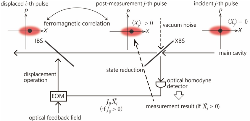
\n ## Diagram: Quantum Measurement Scheme ### Overview This diagram illustrates a quantum measurement scheme involving optical pulses, beam splitters, and a homodyne detector. It depicts the flow of pulses through a main cavity and the process of state reduction based on measurement results. The diagram focuses on the interaction of pulses and the feedback loop involved in the measurement process. ### Components/Axes The diagram features the following components: * **Main Cavity:** A horizontal line representing the main cavity where the pulses propagate. * **IBS (Input Beam Splitter):** A diagonal line with an arrow indicating the splitting of the displaced i-th pulse. * **XBS (Output Beam Splitter):** A diagonal line with an arrow indicating the splitting of the post-measurement j-th pulse. * **EOM (Electro-Optic Modulator):** A rectangular block representing the electro-optic modulator. * **Optical Homodyne Detector:** A rectangular block representing the detector. * **Displaced i-th pulse:** Represented by an elliptical shape with axes labeled 'P' and 'X', indicating momentum and position. * **Post-measurement j-th pulse:** Similar to the displaced pulse, but labeled as post-measurement. * **Incident j-th pulse:** Similar to the displaced pulse, but labeled as incident. * **Arrows:** Indicate the direction of pulse propagation and feedback. * **Labels:** Text annotations describing the components and processes. The diagram uses coordinate axes labeled 'P' (momentum) and 'X' (position) to represent the state of the pulses. ### Detailed Analysis / Content Details The diagram shows the following flow and interactions: 1. **Displaced i-th pulse:** An elliptical shape is positioned to the left of the IBS. The ellipse is oriented diagonally, with axes labeled 'P' and 'X'. A curved arrow above the ellipse indicates "ferromagnetic correlation". 2. **IBS:** The displaced i-th pulse enters the IBS, which splits the pulse. 3. **Main Cavity:** The split pulses propagate through the main cavity (horizontal line). 4. **XBS:** A pulse enters the XBS, which splits the pulse. A dashed line indicates "vacuum noise". 5. **Post-measurement j-th pulse:** An elliptical shape is positioned above the XBS, representing the post-measurement j-th pulse. The ellipse is labeled with "<X> > 0". 6. **Incident j-th pulse:** An elliptical shape is positioned to the right of the XBS, representing the incident j-th pulse. The ellipse is labeled with "<X> = 0". 7. **Optical Homodyne Detector:** The output of the XBS is directed to an optical homodyne detector. 8. **State Reduction:** A dashed arrow indicates "state reduction" from the post-measurement pulse to the detector. 9. **Measurement Result:** The detector output is labeled "measurement result (if X̂ⱼ > 0)". 10. **Feedback Loop:** The detector output is fed back to an EOM via a line labeled "optical feedback field". The EOM output is represented by the equation "Jᵢⱼ X̂ᵢ (if Jᵢⱼ > 0)". 11. **Displacement Operation:** A line labeled "displacement operation" connects the EOM to the input of the IBS. ### Key Observations * The diagram illustrates a feedback loop where the measurement result influences the subsequent pulse displacement. * The state of the pulses changes after measurement, as indicated by the different labels on the post-measurement and incident pulses. * The ferromagnetic correlation suggests a specific type of interaction between the pulses. * The presence of vacuum noise indicates the inherent quantum fluctuations in the system. ### Interpretation This diagram depicts a quantum measurement scheme designed to manipulate and measure the state of optical pulses. The feedback loop, involving the EOM and the optical homodyne detector, suggests a process of continuous measurement and state control. The ferromagnetic correlation and vacuum noise highlight the quantum nature of the system. The state reduction indicates that the measurement process collapses the wave function of the pulse, resulting in a definite measurement outcome. The condition "if Jᵢⱼ > 0" suggests that the feedback is only active when a certain interaction strength is met. The diagram demonstrates a sophisticated approach to quantum measurement, potentially used for quantum information processing or precision sensing. The diagram is a schematic representation of a complex physical setup, and the specific details of the components and interactions would require further information to fully understand.