## Diagram: Octree Expansion and Voxel Insertion ### Overview The image illustrates the process of expanding an octree and inserting points and voxels into it. The process is broken down into five steps: Expand Octree, Sample Voxels, Allocate Chunks, and Insert Points & Voxels. Each step is visually represented with diagrams showing the octree structure and the data being processed. ### Components/Axes * **Title:** Expand Octree and Voxel Insertion * **Steps:** The diagram is divided into 5 steps, numbered 1 through 5. * Step 1: Expand Octree * Step 2: Sample Voxels * Step 3: Allocate Chunks * Step 4: Insert Points & Voxels * **Octree Representation:** The octree is represented as a tree structure with nodes containing numerical values. * **Voxels:** Voxels are represented as small cubes. * **Chunks:** Chunks are represented as rectangular boxes. * **Labels:** * Input * Count * Split ### Detailed Analysis **Step 1: Expand Octree** * **Input:** A single node with the value "0". * **Count:** The node expands to a value of "10", with a cluster of colored spheres above it. * **Split:** The node splits into two child nodes with values "0" and "7", and a third level node with value "3". * **Count:** The tree expands further, with the right branch splitting into nodes "3", "0", "3", and "4". **Step 2: Sample Voxels** * The octree from Step 1 is carried over. * A set of 6 voxels is shown above the tree. * The node with value "4" at the top of the tree is connected to the voxels. * The node with value "2" is connected to two grayed-out nodes. **Step 3: Allocate Chunks** * The octree from Step 2 is carried over. * A set of 6 chunks (rectangular boxes) is shown to the right of the tree. * The nodes with values "4", "2", "3", "3", and "4" are connected to the chunks. **Step 4: Insert Points & Voxels** * The octree from Step 3 is carried over. * The set of 6 voxels is shown above the tree. * The nodes with values "4", "2", "3", "3", and "4" are connected to sets of points and voxels. ### Key Observations * The octree expands from a single node to a more complex tree structure. * Voxels are sampled and allocated to chunks based on the octree structure. * Points and voxels are inserted into the octree based on the allocated chunks. * The numerical values in the nodes seem to represent counts or some other metric related to the data being processed. ### Interpretation The diagram illustrates a hierarchical spatial partitioning process using an octree. The octree is expanded and refined based on the distribution of voxels. Chunks are allocated to the octree nodes, and finally, points and voxels are inserted into the corresponding chunks. This process is commonly used in computer graphics, game development, and scientific visualization for efficient storage and retrieval of spatial data. The diagram provides a high-level overview of the key steps involved in this process.

\n ## Diagram: Octree Processing Pipeline ### Overview The image depicts a four-stage pipeline for processing an octree data structure. The stages are: Expand Octree, Sample Voxels, Allocate Chunks, and Insert Points & Voxels. Each stage visually demonstrates the transformation of data within the octree, with numerical values indicating counts or identifiers. The diagram uses a series of boxes representing octree nodes, arrows indicating data flow, and color-coded icons to represent different data types. ### Components/Axes The diagram is divided into four columns, each representing a stage in the pipeline. Each column has a header indicating the stage name (1. Expand Octree, 2. Sample Voxels, 3. Allocate Chunks, 4. Insert Points & Voxels). Below each header is a visual representation of the octree structure at that stage. The bottom of each column has labels: "Input", "Count", "Split", and "Count". There are also icons at the top of each column representing data types. The icons are: a sphere, a cube, and a collection of smaller cubes. ### Detailed Analysis or Content Details **Stage 1: Expand Octree** * **Input:** A single box labeled "0" with the value "10" below it. * **Split:** The initial box splits into eight smaller boxes. The values within these boxes are: 0, 0, 7, 3, 3, 0, 0, 3. * **Count:** The final "Count" box shows the value "10". **Stage 2: Sample Voxels** * **Input:** The octree structure from Stage 1. * **Sample Voxels:** Several boxes are shaded gray, indicating they are being sampled. The values within the remaining boxes are: 4, 3, 2, 4. * **Count:** The final "Count" box shows the value "4". **Stage 3: Allocate Chunks** * **Input:** The octree structure from Stage 2. * **Allocate Chunks:** Pink rectangles are connected to the octree nodes with arrows, representing chunk allocation. The values within the boxes are: 4, 2, 3, 4. * **Count:** The final "Count" box shows the value "4". **Stage 4: Insert Points & Voxels** * **Input:** The octree structure from Stage 3. * **Insert Points & Voxels:** The octree nodes now contain additional data represented by small, colored squares. The values within the boxes are: 4, 2, 3, 4. * **Count:** The final "Count" box shows the value "4". ### Key Observations * The "Count" value decreases from 10 in the first stage to 4 in the final stage. This suggests a reduction in the number of elements being processed. * The graying out of boxes in Stage 2 indicates a sampling process, potentially filtering or selecting specific voxels. * The pink rectangles in Stage 3 represent the allocation of chunks, likely for memory management or parallel processing. * The addition of colored squares in Stage 4 indicates the insertion of points and voxels into the octree structure. ### Interpretation This diagram illustrates a pipeline for processing octree data, likely for representing 3D space or volumetric data. The pipeline begins by expanding an initial octree node (0) into its eight children. The "Count" value represents the total number of elements within the octree. The subsequent stages involve sampling voxels, allocating chunks, and inserting points and voxels, ultimately resulting in a refined octree structure. The reduction in the "Count" value suggests that the sampling process filters out some voxels, while the chunk allocation and point insertion stages prepare the data for further processing or rendering. The diagram demonstrates a common approach to managing and processing large 3D datasets efficiently. The icons at the top of each stage suggest the data types being handled: a sphere (likely representing a point), a cube (representing a voxel), and a collection of smaller cubes (representing the octree structure itself).

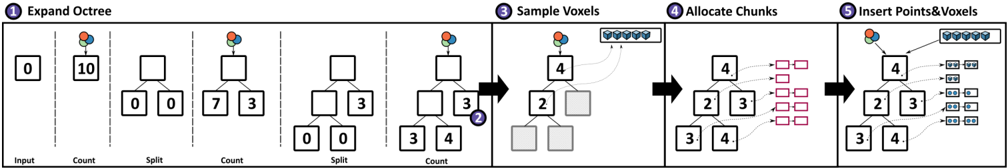
\n ## Technical Diagram: Octree Expansion and Voxel Processing Pipeline ### Overview This image is a technical process diagram illustrating a five-stage pipeline for expanding an octree structure and processing voxel data. The diagram flows horizontally from left to right, with each major stage numbered (1 through 5) and separated by vertical dashed lines or bold arrows. The process involves hierarchical data structures (octrees) and their interaction with voxel grids and memory chunks. ### Components/Axes The diagram is segmented into five sequential stages: 1. **Stage 1: Expand Octree** (Leftmost section, subdivided into 5 sub-steps). 2. **Stage 2: Sample Voxels** (Second section from left). 3. **Stage 3: Allocate Chunks** (Third section from left). 4. **Stage 4: Insert Points & Voxels** (Rightmost section). **Visual Elements:** * **Tree Structures:** Represent octree nodes. Each node is a square box containing a number. * **Numbers:** Integer values within the tree nodes (e.g., 0, 10, 7, 3, 4, 2). * **Spherical Icons:** Clusters of red, green, and blue spheres appear above certain nodes, likely representing point cloud data or voxel samples associated with that node. * **Arrows:** Black arrows indicate the flow of the process between major stages. Thinner, curved arrows within stages show data movement or relationships. * **Grids:** Small square grids (e.g., a 1x8 grid in Stage 2, a 2x4 grid in Stage 4) represent arrays or buffers of voxel data. * **Rectangles:** Pink outlined rectangles in Stage 3 represent allocated memory chunks. * **Icons:** A purple circle with a white 'X' appears in Stage 2, possibly indicating a removed or invalid element. ### Detailed Analysis **Stage 1: Expand Octree** This stage shows the iterative refinement of an octree through a sequence of "Count" and "Split" operations. * **Sub-step 1 (Input):** A single root node containing the value `0`. * **Sub-step 2 (Count):** The root node now contains `10`. A cluster of colored spheres appears above it. * **Sub-step 3 (Split):** The root node is empty. It has two child nodes, both containing `0`. * **Sub-step 4 (Count):** The left child contains `7`, the right child contains `3`. Colored spheres are above the left child. * **Sub-step 5 (Split):** The left child is empty and has two children, both `0`. The right child remains with `3`. * **Sub-step 6 (Count):** The left-most grandchild contains `3`, the right grandchild (from the left child) contains `4`. Colored spheres are above the node with `4`. The right child from the previous split still contains `3`. **Stage 2: Sample Voxels** * Input: The octree state from the end of Stage 1 (a tree with nodes containing values `3`, `4`, and `3`). * Process: A 1x8 grid (blue squares) is shown at the top right. A curved arrow points from this grid to the node containing `4`. * Output: The tree structure is modified. The node that contained `4` now contains `2`. One of its child nodes is a solid grey square (possibly indicating an empty or sampled-out voxel). The purple 'X' icon is placed near the node that previously held a `3` (the right child of the root). **Stage 3: Allocate Chunks** * Input: The modified tree from Stage 2 (nodes with `4`, `2`, `3`, `4`). * Process: Each leaf node with a value (`4`, `2`, `3`, `4`) has a curved arrow pointing to a set of pink outlined rectangles. Each node points to two rectangles, suggesting each node's data is allocated to two memory chunks. **Stage 4: Insert Points & Voxels** * Input: The tree from Stage 3. * Process: The final state of the octree is shown. The node values are `2`, `3`, `4`, and `4`. From each leaf node, arrows point to small data arrays. * The node with `2` points to an array: `[0, 0]`. * The node with `3` points to an array: `[0, 0]`. * The two nodes with `4` point to arrays: `[0, 0]` and `[0, 0]` respectively. * A 2x4 grid of blue squares is shown at the top right, connected to the tree. ### Key Observations 1. **Data Flow:** The pipeline transforms a raw count (`10`) at the root into a refined, spatially partitioned octree where data is distributed to leaf nodes and finally inserted into structured arrays. 2. **Numerical Transformation:** The total count (`10`) is conserved through splits: `7+3=10`, then `3+4+3=10`. In the final stage, the leaf node values (`2, 3, 4, 4`) sum to `13`, which may indicate a change in data representation or the inclusion of new voxel samples from Stage 2. 3. **Visual Anomaly:** The purple 'X' in Stage 2 is a unique icon not repeated elsewhere, highlighting a specific operation (e.g., pruning, error handling, or voxel rejection) at that step. 4. **Spatial Grounding:** The colored sphere clusters are consistently placed above nodes that are actively being processed or hold significant data (the root after first count, a child after split, etc.). The legend for these colors is absent, so their specific meaning (e.g., RGB channels, data types) is inferred but not confirmed. ### Interpretation This diagram details a computational geometry or computer graphics algorithm for managing sparse volumetric data (voxels) using an octree. The process is a classic "divide-and-conquer" strategy: 1. **Expansion (Stage 1):** The octree is built adaptively. Regions with high data density (counts) are recursively subdivided ("Split") to create a more granular spatial index. 2. **Sampling & Allocation (Stages 2 & 3):** The abstract tree structure is connected to concrete data. Voxels are sampled from a source grid, and memory is allocated in chunks corresponding to the leaf nodes of the refined tree. This step bridges the logical spatial partition with physical memory management. 3. **Insertion (Stage 4):** The final step populates the allocated memory with the actual point or voxel data, completing the pipeline from raw input to a structured, query-ready data format. The **purple 'X'** is a critical investigative point. It suggests the algorithm includes a validation or optimization step where certain voxels or tree nodes are discarded, which is essential for handling noise or enforcing constraints in real-world data like 3D scans. The conservation and then apparent increase of the numerical count imply the pipeline integrates multiple data sources (the initial point cloud and the sampled voxel grid). This diagram would be fundamental for engineers implementing a voxel-based renderer, a 3D reconstruction system, or a physics simulation engine dealing with volumetric data.

## Flowchart: Multi-Stage Octree Processing Pipeline ### Overview The image depicts a hierarchical, multi-stage algorithm for processing 3D spatial data using octree decomposition and voxel allocation. The flowchart progresses left-to-right through five distinct phases, with branching logic and data transformations at each step. Color-coded elements (red, blue, green circles; red/blue boxes) represent different data types or processing states. ### Components/Axes 1. **Phases** (Left-to-Right Flow): - Phase 1: Expand Octree - Phase 2: Sample Voxels - Phase 3: Allocate Chunks - Phase 4: Insert Points&Voxels 2. **Key Elements**: - **Input**: Single "0" value - **Count Operations**: Numeric values (10, 7, 3, 4, 2, 3, 4) - **Split Operations**: Binary/ternary divisions (0→0,0; 7→3,4; 3→2,4) - **Voxel Representation**: Blue cubes (6 total) - **Chunk Allocation**: Red/blue boxes (12 total) - **Color-Coded Elements**: - Red circles: Likely root nodes - Blue circles: Leaf nodes - Green circles: Intermediate nodes - Red boxes: Processed chunks - Blue boxes: Raw voxels ### Detailed Analysis 1. **Phase 1: Expand Octree** - Input: Single "0" value - Count: 10 (root node expansion) - Split: 0→0,0 (binary split) - Subsequent splits: 7→3,4; 3→2,4; 4→3,4 2. **Phase 2: Sample Voxels** - Input: 4 (from Phase 1) - Output: 6 blue cubes (voxel sampling) 3. **Phase 3: Allocate Chunks** - Input: 4 (from Phase 2) - Output: 12 boxes (6 red + 6 blue) - Allocation pattern: 4→2,3→3,4 4. **Phase 4: Insert Points&Voxels** - Final output: 12 boxes with embedded blue cubes - Color consistency: Blue boxes retain original voxel data ### Key Observations 1. **Hierarchical Decomposition**: Each split operation reduces node size by factors of 2-4 2. **Data Flow**: Input value 0→10→7→3→4→2→3→4 through successive splits 3. **Memory Allocation**: 1:2 ratio of red (processed) to blue (raw) boxes 4. **Color Consistency**: Blue cubes maintain identity through all phases 5. **Branching Logic**: Each split creates two/three child nodes ### Interpretation This flowchart represents a 3D spatial data processing pipeline with octree-based hierarchical decomposition. The process begins with a single root node (0) that expands through recursive splitting (Phase 1), samples voxels at leaf nodes (Phase 2), allocates memory chunks for storage (Phase 3), and finally inserts processed data into the structure (Phase 4). The consistent use of blue cubes suggests voxel data persistence through transformations, while red boxes indicate processed/optimized data segments. The algorithm appears designed for efficient 3D data management, possibly for applications like 3D rendering, scientific visualization, or spatial database indexing. The color-coding system provides visual cues for data state transitions, with green nodes acting as transitional states between root (red) and leaf (blue) nodes.