## Chart: Cumulative Distribution Function (CDF) of E2E Latency
### Overview
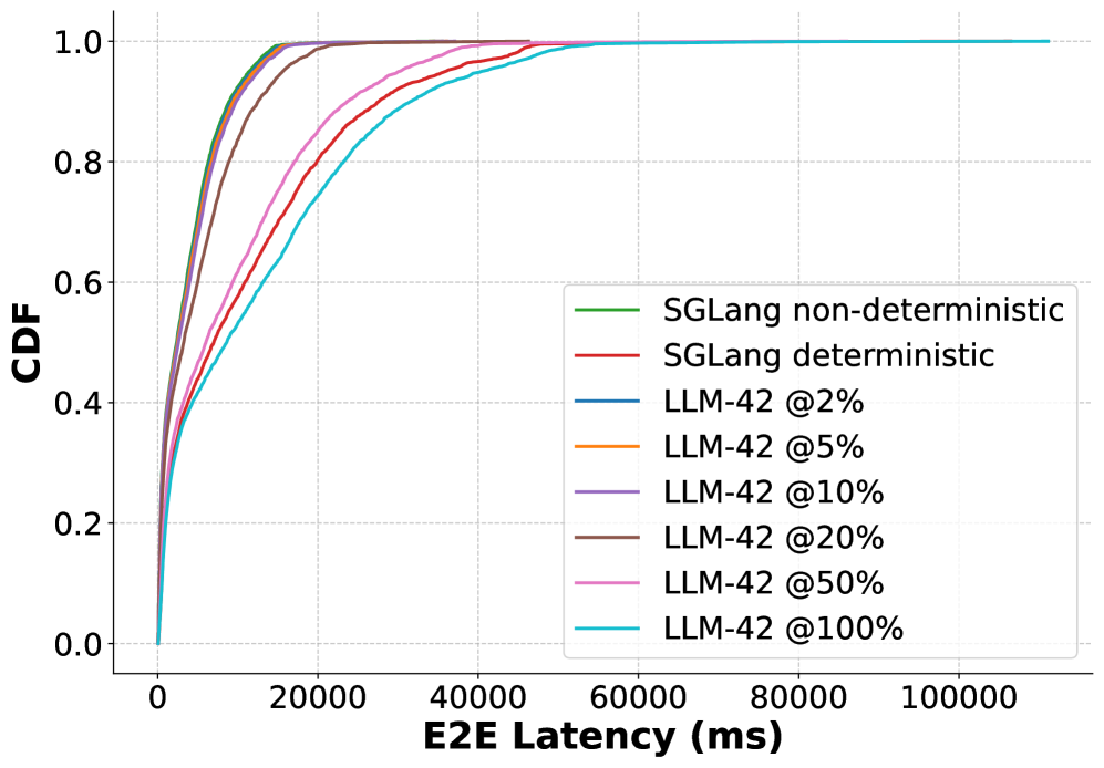
This image displays a Cumulative Distribution Function (CDF) chart comparing the End-to-End (E2E) latency performance of two different systems: **SGLang** (in deterministic and non-deterministic modes) and **LLM-42** (at various percentage configurations ranging from 2% to 100%). The chart illustrates the probability distribution of latency, where a curve positioned further to the left indicates lower latency and better performance.
### Components/Axes
* **X-Axis:** "E2E Latency (ms)". The scale is linear, ranging from 0 to 100,000 ms, with grid lines at 20,000 ms intervals.
* **Y-Axis:** "CDF". The scale is linear, ranging from 0.0 to 1.0, representing the cumulative probability (0% to 100% of requests).
* **Legend:** Located in the center-right region of the chart. It maps colors to specific configurations:
* **Green:** SGLang non-deterministic
* **Red:** SGLang deterministic
* **Blue:** LLM-42 @2%
* **Orange:** LLM-42 @5%
* **Purple:** LLM-42 @10%
* **Brown:** LLM-42 @20%
* **Pink:** LLM-42 @50%
* **Cyan:** LLM-42 @100%
### Detailed Analysis
The data series can be categorized into four distinct performance groups based on their visual trajectory (slope and right-shift):
1. **High-Performance Group (Green, Red, Blue, Orange, Purple):**
* **Trend:** These lines are tightly clustered and exhibit the steepest upward slope, indicating the lowest latency.
* **Median (0.5 CDF):** Approximately 5,000 ms.
* **90th Percentile (0.9 CDF):** Approximately 12,000 ms.
* **Max Latency:** These configurations reach 1.0 CDF at approximately 20,000 ms.
2. **Moderate-Performance Group (Brown - LLM-42 @20%):**
* **Trend:** This line shifts to the right of the high-performance group, indicating higher latency.
* **Median (0.5 CDF):** Approximately 8,000 ms.
* **90th Percentile (0.9 CDF):** Approximately 25,000 ms.
* **Max Latency:** Reaches 1.0 CDF at approximately 45,000 ms.
3. **Lower-Performance Group (Pink - LLM-42 @50%):**
* **Trend:** Further right-shift compared to the 20% configuration.
* **Median (0.5 CDF):** Approximately 10,000 ms.
* **90th Percentile (0.9 CDF):** Approximately 30,000 ms.
* **Max Latency:** Reaches 1.0 CDF at approximately 50,000 ms.
4. **Lowest-Performance Group (Cyan - LLM-42 @100%):**
* **Trend:** This is the right-most curve, indicating the highest latency.
* **Median (0.5 CDF):** Approximately 12,000 ms.
* **90th Percentile (0.9 CDF):** Approximately 40,000 ms.
* **Max Latency:** Reaches 1.0 CDF at approximately 110,000 ms.
### Key Observations
* **Performance Scaling:** There is a clear correlation between the LLM-42 percentage parameter and latency. As the percentage increases from 2% to 100%, the latency distribution shifts significantly to the right, indicating a degradation in performance.
* **SGLang Efficiency:** Both SGLang configurations (deterministic and non-deterministic) perform at the same level as the lowest-load LLM-42 configurations (2%, 5%, 10%), suggesting high efficiency.
* **Tail Latency:** The divergence between the configurations is most pronounced at the higher end of the CDF (approaching 1.0). While the median latency differences are relatively small (ranging from ~5s to ~12s), the maximum latency differences are massive (ranging from ~20s to ~110s).
### Interpretation
The data demonstrates that the LLM-42 system experiences significant performance degradation as the load or complexity (represented by the percentage parameter) increases. The "100%" configuration is an outlier in terms of tail latency, taking over five times longer to complete the slowest requests compared to the SGLang baseline.
From a technical standpoint, this suggests that the LLM-42 system may have non-linear scaling issues or resource contention problems as the workload increases. Conversely, SGLang maintains a tight, predictable latency profile regardless of its deterministic or non-deterministic mode, making it the superior choice for latency-sensitive applications based on this specific dataset.