## Chart: Cumulative Distribution Function of E2E Latency
### Overview
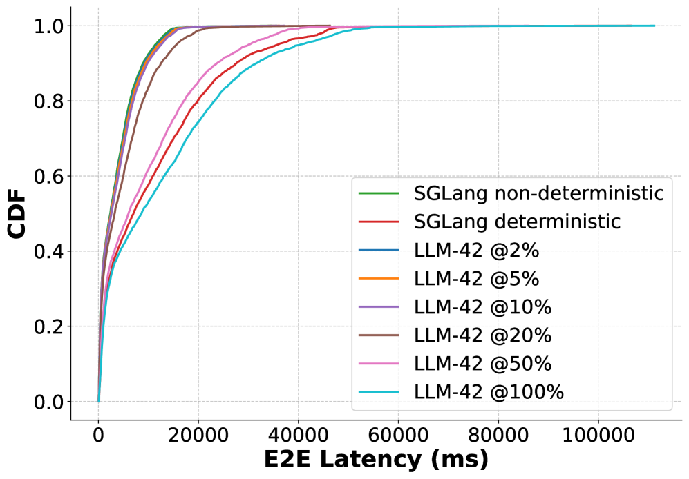
The image presents a cumulative distribution function (CDF) plot illustrating the end-to-end (E2E) latency of different language models. The x-axis represents latency in milliseconds (ms), and the y-axis represents the cumulative distribution function (CDF), ranging from 0.0 to 1.0. Several lines are plotted, each representing a different model or configuration.
### Components/Axes
* **X-axis Title:** E2E Latency (ms)
* **Y-axis Title:** CDF
* **Legend:** Located in the top-right corner, listing the following data series:
* SGLang non-deterministic (Green)
* SGLang deterministic (Red)
* LLM-42 @2% (Blue)
* LLM-42 @5% (Orange)
* LLM-42 @10% (Purple)
* LLM-42 @20% (Brown)
* LLM-42 @50% (Pink)
* LLM-42 @100% (Light Blue)
* **Gridlines:** A light gray grid is present to aid in reading values.
* **Axis Scale:** X-axis ranges from approximately 0 to 100000 ms. Y-axis ranges from 0.0 to 1.0.
### Detailed Analysis
The chart displays the CDF for several models. Here's a breakdown of each line's trend and approximate data points:
* **SGLang non-deterministic (Green):** This line starts at approximately CDF 0.0 at E2E Latency 0 ms, rises sharply to CDF 0.8 at approximately 10000 ms, and reaches CDF 1.0 at around 25000 ms.
* **SGLang deterministic (Red):** This line starts at approximately CDF 0.0 at E2E Latency 0 ms, rises sharply to CDF 0.8 at approximately 15000 ms, and reaches CDF 1.0 at around 30000 ms.
* **LLM-42 @2% (Blue):** This line starts at approximately CDF 0.0 at E2E Latency 0 ms, rises to CDF 0.8 at approximately 30000 ms, and reaches CDF 1.0 at around 60000 ms.
* **LLM-42 @5% (Orange):** This line starts at approximately CDF 0.0 at E2E Latency 0 ms, rises to CDF 0.8 at approximately 35000 ms, and reaches CDF 1.0 at around 70000 ms.
* **LLM-42 @10% (Purple):** This line starts at approximately CDF 0.0 at E2E Latency 0 ms, rises to CDF 0.8 at approximately 40000 ms, and reaches CDF 1.0 at around 80000 ms.
* **LLM-42 @20% (Brown):** This line starts at approximately CDF 0.0 at E2E Latency 0 ms, rises to CDF 0.8 at approximately 45000 ms, and reaches CDF 1.0 at around 90000 ms.
* **LLM-42 @50% (Pink):** This line starts at approximately CDF 0.0 at E2E Latency 0 ms, rises to CDF 0.8 at approximately 50000 ms, and reaches CDF 1.0 at around 95000 ms.
* **LLM-42 @100% (Light Blue):** This line starts at approximately CDF 0.0 at E2E Latency 0 ms, rises to CDF 0.8 at approximately 55000 ms, and reaches CDF 1.0 at around 100000 ms.
### Key Observations
* The SGLang models (both deterministic and non-deterministic) exhibit significantly lower latency compared to the LLM-42 models.
* As the percentage increases in the LLM-42 models (@2% to @100%), the latency generally increases. This is evident in the rightward shift of the CDF curves.
* The deterministic SGLang model has slightly higher latency than the non-deterministic version.
* The LLM-42 models show a relatively consistent increase in latency as the percentage parameter increases.
### Interpretation
This chart demonstrates the trade-off between latency and potentially other factors (like accuracy or complexity) in different language models. The SGLang models are faster, suggesting they might be simpler or optimized for speed. The LLM-42 models, while slower, offer a range of configurations (represented by the percentages) that allow for tuning the latency based on application requirements. The CDF plot is useful for understanding the probability of observing a particular latency value for each model. For example, the chart shows that the LLM-42 @2% model has a 50% probability of completing within approximately 30000 ms, while the LLM-42 @100% model has a 50% probability of completing within approximately 55000 ms. The increasing latency with higher percentages in LLM-42 likely indicates increased computational cost associated with more complex processing or larger model sizes.