## Phase Portrait: Vector Field Around an Equilibrium Point
### Overview
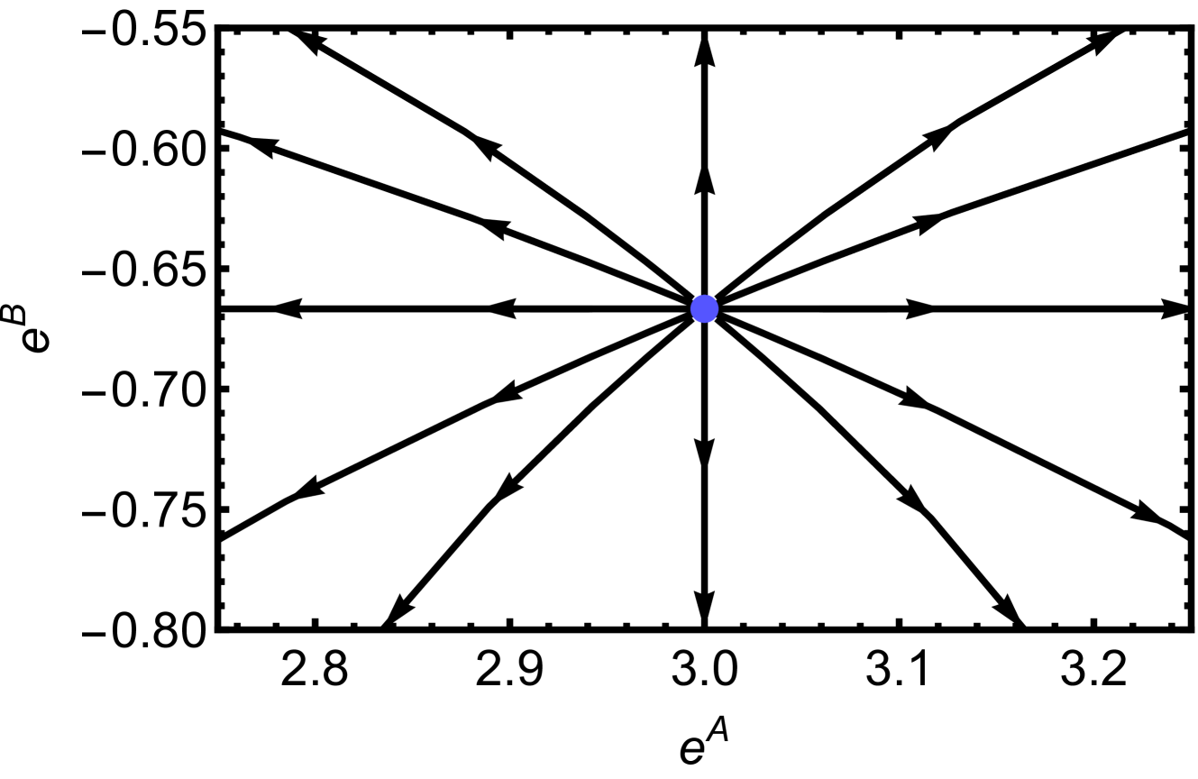
The image is a 2D phase portrait or vector field plot, likely from the study of dynamical systems. It visualizes the direction of flow or trajectories in a state space defined by two variables, `e^A` and `e^B`. The plot is centered on a single, distinct equilibrium point, with arrows indicating the direction of movement for states near that point.
### Components/Axes
* **Chart Type:** 2D Vector Field / Phase Portrait.
* **Horizontal Axis (X-axis):**
* **Label:** `e^A`
* **Scale:** Linear.
* **Range:** Approximately 2.75 to 3.25.
* **Major Tick Marks:** 2.8, 2.9, 3.0, 3.1, 3.2.
* **Vertical Axis (Y-axis):**
* **Label:** `e^B`
* **Scale:** Linear.
* **Range:** Approximately -0.80 to -0.55.
* **Major Tick Marks:** -0.80, -0.75, -0.70, -0.65, -0.60, -0.55.
* **Central Element:**
* A solid blue dot located at the intersection of the axes' central values.
* **Coordinates:** `(e^A, e^B) ≈ (3.0, -0.67)`. This is the system's fixed or equilibrium point.
* **Vector Field:**
* Composed of 12 black arrows of uniform length and style.
* All arrows originate from or point directly toward the central blue dot, indicating the local dynamics around the equilibrium.
* **Spatial Arrangement:** The arrows are arranged radially around the central point, with one arrow aligned with each major axis direction (up, down, left, right) and one arrow in each of the four diagonal quadrants.
### Detailed Analysis
* **Axis Data Points:**
* `e^A` axis markers: 2.8, 2.9, 3.0, 3.1, 3.2.
* `e^B` axis markers: -0.80, -0.75, -0.70, -0.65, -0.60, -0.55.
* **Equilibrium Point:** The system has a single fixed point at approximately `(3.0, -0.67)`.
* **Vector Directions (Trend Verification):**
* **Arrows Pointing INWARD (Toward the blue dot):**
* The arrow pointing **left** (along the negative `e^A` direction from the center).
* The arrow pointing **down** (along the negative `e^B` direction from the center).
* The arrow pointing **down-left** (into the third quadrant relative to the center).
* The arrow pointing **down-right** (into the fourth quadrant relative to the center).
* **Arrows Pointing OUTWARD (Away from the blue dot):**
* The arrow pointing **right** (along the positive `e^A` direction from the center).
* The arrow pointing **up** (along the positive `e^B` direction from the center).
* The arrow pointing **up-left** (into the second quadrant relative to the center).
* The arrow pointing **up-right** (into the first quadrant relative to the center).
* **Neutral/Aligned Arrows:** The arrows pointing directly **left** and **right** are perfectly horizontal. The arrows pointing directly **up** and **down** are perfectly vertical.
### Key Observations
1. **Saddle Point Dynamics:** The pattern of arrows—some pointing toward the equilibrium along one axis (the `e^B` axis and the down-left/down-right diagonals) and others pointing away along another axis (the `e^A` axis and the up-left/up-right diagonals)—is the classic signature of a **saddle point** in a dynamical system.
2. **Stable and Unstable Manifolds:**
* The **vertical axis (`e^B`)** and the two downward diagonal directions appear to be part of the **stable manifold**. Trajectories along these directions approach the equilibrium.
* The **horizontal axis (`e^A`)** and the two upward diagonal directions appear to be part of the **unstable manifold**. Trajectories along these directions move away from the equilibrium.
3. **Symmetry:** The vector field exhibits a high degree of symmetry about the central point, particularly reflection symmetry across both the vertical and horizontal axes passing through `(3.0, -0.67)`.
4. **No Legend:** The chart contains no separate legend. The meaning of the arrows (direction of flow) and the blue dot (equilibrium) is inferred from standard conventions in phase portrait diagrams.
### Interpretation
This phase portrait illustrates the local behavior of a two-dimensional dynamical system near a saddle-type equilibrium point. The variables `e^A` and `e^B` could represent error terms, state variables, or concentrations in a model.
* **What the data suggests:** The system is unstable at the point `(3.0, -0.67)`. While a state exactly on the stable manifold (the vertical line `e^A = 3.0` or the specific downward diagonals) would theoretically converge to the equilibrium, any slight perturbation will cause the state to be pushed away along the unstable manifold (the horizontal line `e^B = -0.67` or the upward diagonals). In practical terms, this equilibrium is not physically observable; the system will not settle there.
* **Relationship between elements:** The central blue dot defines the point of balance. The arrows map out the "force field" or velocity vector at sample points around it, revealing the underlying structure of the system's differential equations. The direction of each arrow is determined by the system's equations of motion evaluated at that point in the `(e^A, e^B)` plane.
* **Notable Anomalies:** There are no outliers in the traditional data sense. The pattern is highly regular and mathematically consistent with a linearized system around a saddle point. The key "anomaly" is the existence of the saddle point itself, which dictates that most nearby trajectories will eventually diverge from this region of the state space.