## Scatter Plot: Model Accuracy vs. Compute (Normalized FLOPs)
### Overview
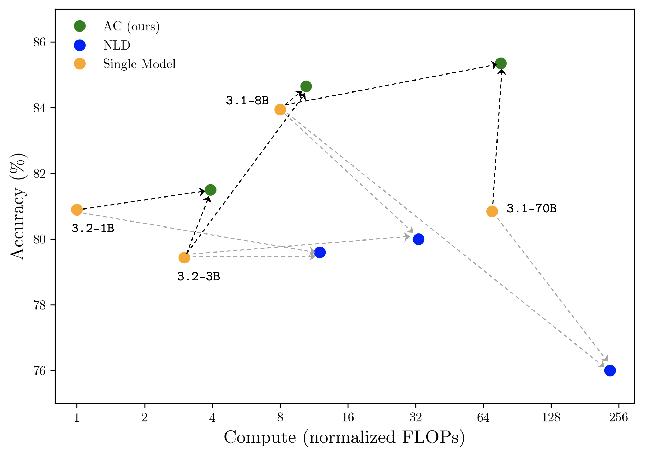
This is a scatter plot comparing the performance of three different model types or methods—labeled "AC (ours)", "NLD", and "Single Model"—across two dimensions: computational cost (x-axis) and accuracy (y-axis). The plot uses a logarithmic scale for the x-axis. Data points for the "Single Model" category are explicitly labeled with model names (e.g., "3.2-1B"). Dashed lines with arrows connect points, indicating a directional relationship or transition between model versions or configurations.
### Components/Axes
* **X-Axis:** Labeled "Compute (normalized FLOPs)". It is a logarithmic scale with major tick marks at 1, 2, 4, 8, 16, 32, 64, 128, and 256.
* **Y-Axis:** Labeled "Accuracy (%)". It is a linear scale ranging from approximately 75% to 87%, with major tick marks at 76, 78, 80, 82, 84, and 86.
* **Legend:** Located in the top-left corner of the plot area.
* **Green Circle:** "AC (ours)"
* **Blue Circle:** "NLD"
* **Orange Circle:** "Single Model"
* **Data Point Labels:** Four orange "Single Model" points have text labels placed directly below or beside them:
* "3.2-1B" (leftmost orange point)
* "3.2-3B" (second orange point from left)
* "3.1-8B" (third orange point from left)
* "3.1-70B" (rightmost orange point)
### Detailed Analysis
**Data Series and Approximate Points:**
1. **Single Model (Orange Circles):**
* **Trend:** The points show a non-monotonic relationship. Accuracy initially dips from the 1B to 3B model, then rises sharply for the 8B model, before falling again for the 70B model.
* **Points (Compute, Accuracy):**
* 3.2-1B: (~1, ~80.9%)
* 3.2-3B: (~3, ~79.5%)
* 3.1-8B: (~8, ~84.0%)
* 3.1-70B: (~70, ~80.9%)
2. **AC (ours) (Green Circles):**
* **Trend:** Shows a consistent upward trend. As compute increases, accuracy increases.
* **Points (Compute, Accuracy):**
* Point 1: (~4, ~81.5%)
* Point 2: (~10, ~84.6%)
* Point 3: (~80, ~85.3%)
3. **NLD (Blue Circles):**
* **Trend:** Shows a consistent downward trend. As compute increases, accuracy decreases.
* **Points (Compute, Accuracy):**
* Point 1: (~12, ~79.6%)
* Point 2: (~32, ~80.0%)
* Point 3: (~240, ~76.0%)
**Connections (Dashed Lines with Arrows):**
* **Black Dashed Lines (with arrows pointing to Green/AC points):** These lines connect each orange "Single Model" point to a corresponding green "AC (ours)" point that is positioned at a higher accuracy and, in two cases, higher compute. This visually suggests that the "AC" method improves upon the base "Single Model".
* 3.2-1B (Orange) → AC Point 1 (Green)
* 3.2-3B (Orange) → AC Point 1 (Green) *[Note: Two orange points connect to the same green point]*
* 3.1-8B (Orange) → AC Point 2 (Green)
* 3.1-70B (Orange) → AC Point 3 (Green)
* **Grey Dashed Lines (with arrows pointing to Blue/NLD points):** These lines connect each orange "Single Model" point to a corresponding blue "NLD" point. The relationship is mixed: for the 1B and 3B models, the NLD point is at similar or slightly lower accuracy but higher compute. For the 8B and 70B models, the NLD point is at significantly lower accuracy and higher compute.
* 3.2-1B (Orange) → NLD Point 1 (Blue)
* 3.2-3B (Orange) → NLD Point 1 (Blue) *[Note: Two orange points connect to the same blue point]*
* 3.1-8B (Orange) → NLD Point 2 (Blue)
* 3.1-70B (Orange) → NLD Point 3 (Blue)
### Key Observations
1. **Performance Hierarchy:** At every connected comparison point, the "AC (ours)" method achieves higher accuracy than its corresponding "Single Model" baseline. The "NLD" method generally performs worse than or comparable to the "Single Model" baseline, with a severe drop in accuracy for the highest-compute configuration.
2. **Scaling Behavior:** The three methods exhibit fundamentally different scaling properties with respect to compute:
* **AC (ours):** Positive scaling (more compute → higher accuracy).
* **NLD:** Negative scaling (more compute → lower accuracy).
* **Single Model:** Irregular scaling, with a peak at the 8B parameter model.
3. **Efficiency:** The "AC" method appears to be the most compute-efficient for achieving high accuracy. For example, the AC point at ~10 normalized FLOPs achieves ~84.6% accuracy, surpassing the best Single Model (3.1-8B at ~84.0%) with only a modest increase in compute.
4. **Outlier:** The "NLD" point at ~240 normalized FLOPs is a significant outlier, showing the lowest accuracy (~76.0%) on the chart despite using the most compute.
### Interpretation
This chart is likely from a research paper proposing a new model training or architecture method called "AC" (the authors' method). It demonstrates the method's superiority over two baselines: a standard "Single Model" approach and another method called "NLD".
The core message is one of **improved scaling and efficiency**. The "AC" method successfully translates increased computational resources (normalized FLOPs) into higher task accuracy, which is the desired behavior for scalable AI systems. In contrast, the "NLD" method exhibits pathological scaling, where throwing more compute at the problem actually harms performance, suggesting instability or a fundamental mismatch between the method and the scaling axis.
The irregular performance of the "Single Model" baseline (dipping at 3B, peaking at 8B) might reflect challenges in training stability or data requirements at different model scales. The "AC" method appears to smooth out this irregularity, providing a more reliable performance improvement over the baseline across the scale spectrum.
The arrows are critical: they don't just show data points; they tell a story of **transformation**. They visually argue that applying the "AC" technique to a base model (orange) reliably "lifts" it to a higher-performing state (green), while applying "NLD" often "drags" it down (blue). This makes a compelling case for the adoption of the "AC" method.