## Scatter Plot: Accuracy vs. Lambda Squared
### Overview
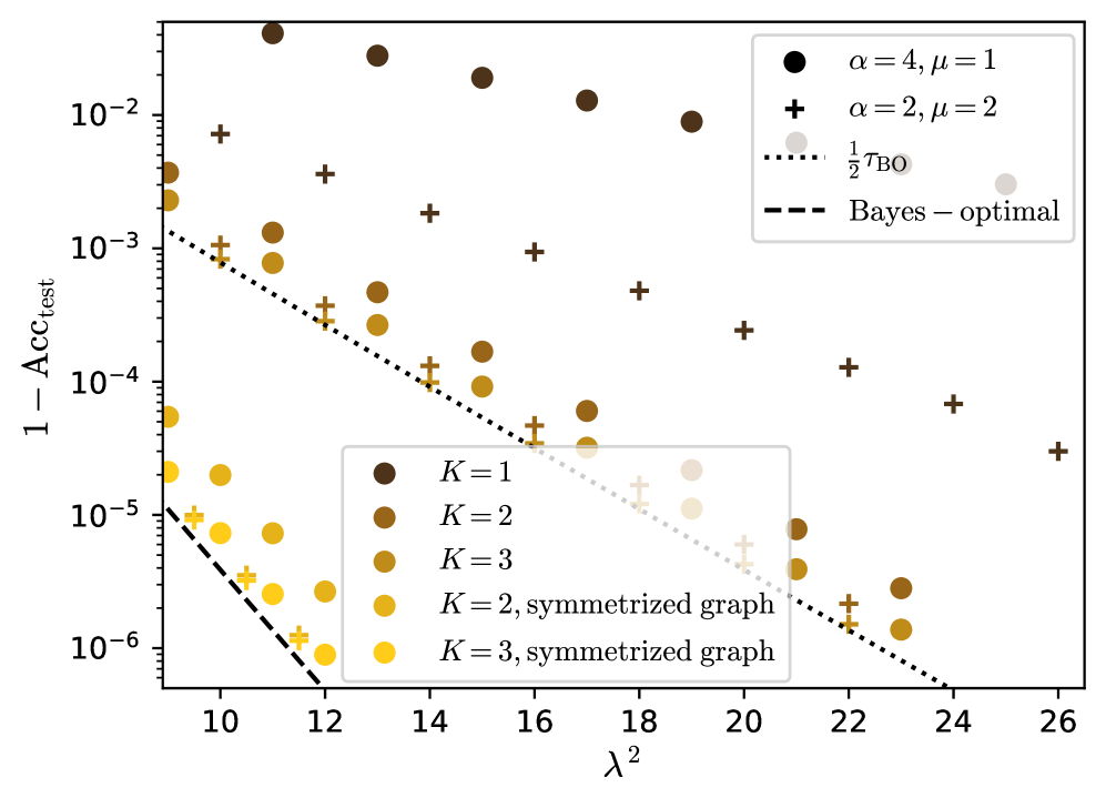
The image is a scatter plot showing the relationship between `1 - Acc_test` (error rate) and `λ^2` (lambda squared). The plot includes multiple data series, each representing different configurations of parameters `K`, `α`, and `μ`, as well as two reference lines: `1/2 τ_BO` and `Bayes-optimal`. The y-axis is on a logarithmic scale.
### Components/Axes
* **X-axis:** `λ^2` (lambda squared), with a linear scale ranging from approximately 9 to 26.
* **Y-axis:** `1 - Acc_test` (error rate), with a logarithmic scale ranging from 10^-6 to 10^-2.
* **Legend (Top-Right):**
* Black circle: `α = 4, μ = 1`
* Black plus sign: `α = 2, μ = 2`
* Dotted line: `1/2 τ_BO`
* Dashed line: `Bayes - optimal`
* **Legend (Center):**
* Dark brown circle: `K = 1`
* Brown circle: `K = 2`
* Dark yellow circle: `K = 3`
* Yellow circle: `K = 2, symmetrized graph`
* Light yellow circle: `K = 3, symmetrized graph`
### Detailed Analysis
* **Data Series: `α = 4, μ = 1` (Black Circles)**
* Trend: The error rate decreases as `λ^2` increases.
* Data Points:
* λ^2 = 10, 1 - Acc_test ≈ 0.015
* λ^2 = 16, 1 - Acc_test ≈ 0.008
* λ^2 = 22, 1 - Acc_test ≈ 0.006
* λ^2 = 26, 1 - Acc_test ≈ 0.005
* **Data Series: `α = 2, μ = 2` (Black Plus Signs)**
* Trend: The error rate decreases as `λ^2` increases.
* Data Points:
* λ^2 = 10, 1 - Acc_test ≈ 0.006
* λ^2 = 16, 1 - Acc_test ≈ 0.002
* λ^2 = 22, 1 - Acc_test ≈ 0.0005
* λ^2 = 26, 1 - Acc_test ≈ 0.0003
* **Data Series: `K = 1` (Dark Brown Circles)**
* Trend: The error rate decreases as `λ^2` increases.
* Data Points:
* λ^2 = 10, 1 - Acc_test ≈ 0.004
* λ^2 = 16, 1 - Acc_test ≈ 0.0004
* λ^2 = 22, 1 - Acc_test ≈ 0.00008
* **Data Series: `K = 2` (Brown Circles)**
* Trend: The error rate decreases as `λ^2` increases.
* Data Points:
* λ^2 = 10, 1 - Acc_test ≈ 0.001
* λ^2 = 16, 1 - Acc_test ≈ 0.0001
* λ^2 = 22, 1 - Acc_test ≈ 0.00002
* **Data Series: `K = 3` (Dark Yellow Circles)**
* Trend: The error rate decreases as `λ^2` increases.
* Data Points:
* λ^2 = 10, 1 - Acc_test ≈ 0.0002
* λ^2 = 16, 1 - Acc_test ≈ 0.00003
* λ^2 = 22, 1 - Acc_test ≈ 0.000006
* **Data Series: `K = 2, symmetrized graph` (Yellow Circles)**
* Trend: The error rate decreases as `λ^2` increases.
* Data Points:
* λ^2 = 10, 1 - Acc_test ≈ 0.00002
* λ^2 = 16, 1 - Acc_test ≈ 0.000004
* λ^2 = 22, 1 - Acc_test ≈ 0.000001
* **Data Series: `K = 3, symmetrized graph` (Light Yellow Circles)**
* Trend: The error rate decreases as `λ^2` increases.
* Data Points:
* λ^2 = 10, 1 - Acc_test ≈ 0.000005
* λ^2 = 16, 1 - Acc_test ≈ 0.000001
* λ^2 = 22, 1 - Acc_test ≈ 0.0000003
* **Reference Line: `1/2 τ_BO` (Dotted Line)**
* Trend: Decreases as `λ^2` increases.
* At λ^2 = 10, 1 - Acc_test ≈ 0.001
* At λ^2 = 26, 1 - Acc_test ≈ 0.000001
* **Reference Line: `Bayes - optimal` (Dashed Line)**
* Trend: Decreases as `λ^2` increases.
* At λ^2 = 10, 1 - Acc_test ≈ 0.00001
* At λ^2 = 12, 1 - Acc_test ≈ 0.000001
### Key Observations
* The error rate (`1 - Acc_test`) generally decreases as `λ^2` increases across all data series.
* The data series with higher `α` and lower `μ` (black circles) generally have higher error rates compared to those with lower `α` and higher `μ` (black plus signs).
* Symmetrizing the graph (yellow and light yellow circles) results in lower error rates compared to the non-symmetrized versions (brown and dark yellow circles) for the same `K` value.
* Increasing `K` generally leads to lower error rates.
* The `Bayes - optimal` line represents the lowest achievable error rate, and all data series approach this limit as `λ^2` increases.
### Interpretation
The plot illustrates the impact of different parameters (`α`, `μ`, `K`) and graph symmetrization on the test accuracy of a model as a function of `λ^2`. The decreasing error rates with increasing `λ^2` suggest that higher regularization (represented by `λ^2`) improves the model's generalization performance. The comparison between different parameter configurations highlights the trade-offs between model complexity and accuracy. Symmetrizing the graph appears to be an effective technique for reducing the error rate. The plot also demonstrates how the model's performance approaches the theoretical `Bayes - optimal` limit with increasing regularization.