## Line Chart: Effect of Time Step (CIM-CAC)
### Overview
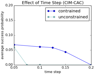
This is a line chart titled "Effect of Time Step (CIM-CAC)". It plots the relationship between a "time step" variable on the horizontal axis and the "average success probability" on the vertical axis. The chart compares two conditions or models: "constrained" and "unconstrained".
### Components/Axes
* **Chart Title:** "Effect of Time Step (CIM-CAC)" (centered at the top).
* **Y-Axis:**
* **Label:** "average success probability" (rotated vertically on the left).
* **Scale:** Linear scale ranging from 0.00 to 0.20.
* **Major Ticks:** 0.00, 0.05, 0.10, 0.15, 0.20.
* **X-Axis:**
* **Label:** "time step" (centered at the bottom).
* **Scale:** Linear scale ranging from 0.05 to 0.2.
* **Major Ticks:** 0.05, 0.1, 0.15, 0.2.
* **Legend:**
* **Position:** Top-right corner of the plot area.
* **Items:**
1. **Blue line with circle markers:** Labeled "constrained".
2. **Teal (light blue-green) line with circle markers:** Labeled "unconstrained".
### Detailed Analysis
**Data Series 1: "constrained" (Blue Line)**
* **Trend:** The line shows a gradual, monotonic downward slope. It starts at a moderate success probability and declines steadily as the time step increases, reaching zero at the final measured point.
* **Data Points (Approximate):**
* At time step `0.05`: average success probability ≈ `0.065`
* At time step `0.1`: average success probability ≈ `0.060`
* At time step `0.125`: average success probability ≈ `0.058`
* At time step `0.15`: average success probability ≈ `0.045`
* At time step `0.2`: average success probability = `0.00`
**Data Series 2: "unconstrained" (Teal Line)**
* **Trend:** The line shows a very sharp, immediate decline. It starts at a success probability similar to the constrained case at the smallest time step but plummets to zero almost immediately and remains there.
* **Data Points (Approximate):**
* At time step `0.05`: average success probability ≈ `0.050`
* At time step `0.075` (inferred between 0.05 and 0.1): average success probability ≈ `0.00`
* At time step `0.1`: average success probability = `0.00`
* At time step `0.15`: average success probability = `0.00`
* At time step `0.2`: average success probability = `0.00`
### Key Observations
1. **Divergent Degradation:** The two conditions exhibit fundamentally different failure modes. The "constrained" system degrades gracefully, while the "unconstrained" system fails catastrophically and immediately.
2. **Critical Threshold:** For the "unconstrained" model, the success probability drops to zero at a time step value between `0.05` and `0.075`. This suggests a very low tolerance for increased time steps.
3. **Constrained Resilience:** The "constrained" model maintains a non-zero success probability for a much wider range of time steps, only failing completely at `0.2`.
4. **Initial Performance:** At the smallest measured time step (`0.05`), the "constrained" model already shows a higher average success probability (~0.065) than the "unconstrained" model (~0.050).
### Interpretation
The chart demonstrates a clear performance trade-off related to system constraints in the context of the CIM-CAC model or experiment. The data suggests that applying constraints ("constrained" condition) significantly improves the system's robustness to increases in the "time step" parameter.
* **The "unconstrained" system** appears highly sensitive. Even a small increase in time step from 0.05 leads to a complete loss of success probability. This could indicate instability, a lack of error correction, or a propensity for rapid divergence when not bound by specific rules.
* **The "constrained" system** exhibits stability and predictability. Its performance decays in a controlled, near-linear fashion. The constraints likely enforce an operational envelope that prevents catastrophic failure, allowing the system to function, albeit with diminishing returns, over a broader operational range.
**Underlying Implication:** In the context of whatever process "CIM-CAC" represents (e.g., a computational algorithm, a control system, a simulation), incorporating constraints is not a limitation but a necessary design feature for achieving operational resilience and extending the viable parameter space. The "unconstrained" approach, while perhaps simpler, is practically unusable for any time step beyond the minimal value. The chart argues for the necessity of the constrained design.