\n
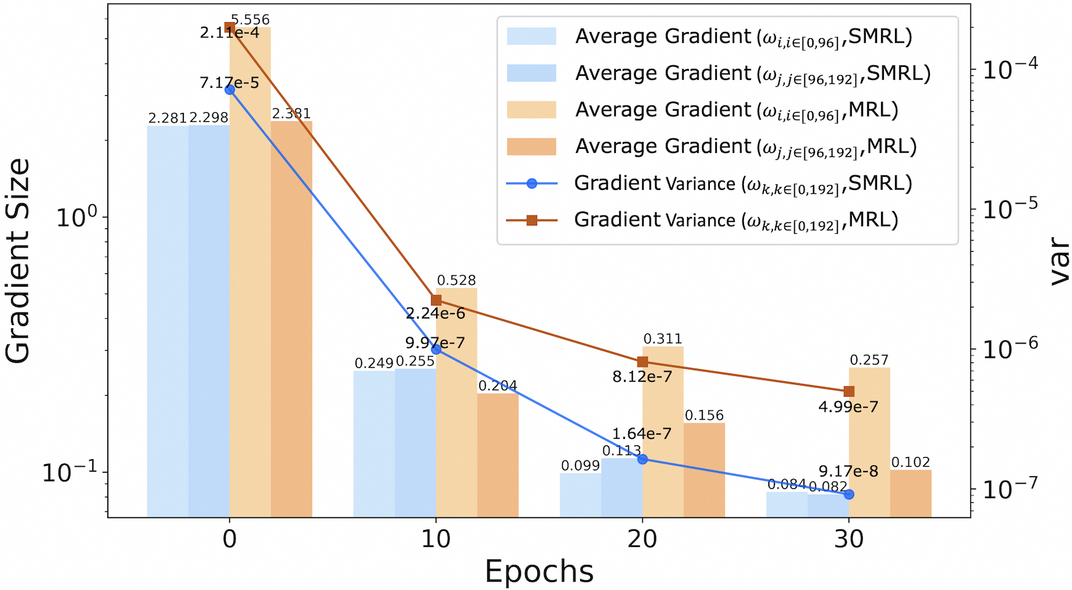
## Combination Bar and Line Chart: Gradient Size and Variance Across Epochs for SMRL and MRL
### Overview
This image is a technical chart comparing gradient statistics between two methods, SMRL and MRL, over the course of training epochs. It uses a dual-axis format: the primary (left) y-axis shows "Gradient Size" on a logarithmic scale, and the secondary (right) y-axis shows "var" (variance), also on a logarithmic scale. The x-axis represents training "Epochs". The chart combines grouped bar plots for average gradient magnitudes and line plots for gradient variance.
### Components/Axes
* **X-Axis:** Labeled "Epochs". Major tick marks and labels are at values 0, 10, 20, and 30.
* **Primary Y-Axis (Left):** Labeled "Gradient Size". It is a logarithmic scale with major ticks at 10⁻¹ (0.1) and 10⁰ (1).
* **Secondary Y-Axis (Right):** Labeled "var". It is a logarithmic scale with major ticks at 10⁻⁷, 10⁻⁶, 10⁻⁵, and 10⁻⁴.
* **Legend:** Located in the top-right quadrant of the chart. It defines six data series:
1. **Light Blue Bar:** `Average Gradient (ω_i, i∈[0,96], SMRL)`
2. **Medium Blue Bar:** `Average Gradient (ω_j, j∈[96,192], SMRL)`
3. **Light Orange Bar:** `Average Gradient (ω_i, i∈[0,96], MRL)`
4. **Medium Orange Bar:** `Average Gradient (ω_j, j∈[96,192], MRL)`
5. **Blue Line with Circle Markers:** `Gradient Variance (ω_k, k∈[0,192], SMRL)`
6. **Brown Line with Square Markers:** `Gradient Variance (ω_k, k∈[0,192], MRL)`
### Detailed Analysis
Data is presented at four discrete epochs: 0, 10, 20, and 30. Values are approximate, read from the chart annotations.
**Epoch 0:**
* **Bars (Gradient Size):**
* SMRL (ω_i, [0,96]): ~2.281
* SMRL (ω_j, [96,192]): ~2.298
* MRL (ω_i, [0,96]): ~5.556
* MRL (ω_j, [96,192]): ~2.381
* **Lines (Variance):**
* SMRL Variance: ~7.17e-5 (Blue circle)
* MRL Variance: ~2.11e-4 (Brown square)
**Epoch 10:**
* **Bars (Gradient Size):**
* SMRL (ω_i, [0,96]): ~0.249
* SMRL (ω_j, [96,192]): ~0.255
* MRL (ω_i, [0,96]): ~0.528
* MRL (ω_j, [96,192]): ~0.204
* **Lines (Variance):**
* SMRL Variance: ~9.97e-7 (Blue circle)
* MRL Variance: ~2.24e-6 (Brown square)
**Epoch 20:**
* **Bars (Gradient Size):**
* SMRL (ω_i, [0,96]): ~0.099
* SMRL (ω_j, [96,192]): ~0.113
* MRL (ω_i, [0,96]): ~0.311
* MRL (ω_j, [96,192]): ~0.156
* **Lines (Variance):**
* SMRL Variance: ~1.64e-7 (Blue circle)
* MRL Variance: ~8.12e-7 (Brown square)
**Epoch 30:**
* **Bars (Gradient Size):**
* SMRL (ω_i, [0,96]): ~0.084
* SMRL (ω_j, [96,192]): ~0.082
* MRL (ω_i, [0,96]): ~0.257
* MRL (ω_j, [96,192]): ~0.102
* **Lines (Variance):**
* SMRL Variance: ~9.17e-8 (Blue circle)
* MRL Variance: ~4.99e-7 (Brown square)
### Key Observations
1. **Overall Trend:** All metrics (average gradient size for both weight groups and both methods, and gradient variance for both methods) show a clear, consistent downward trend from Epoch 0 to Epoch 30.
2. **Method Comparison (Gradient Size):** At every epoch, the average gradient sizes for MRL (orange bars) are larger than their SMRL (blue bar) counterparts for the same weight group (i∈[0,96] or j∈[96,192]). The difference is most pronounced at Epoch 0.
3. **Method Comparison (Variance):** The gradient variance for MRL (brown line) is consistently higher than for SMRL (blue line) at all measured epochs. The gap between them narrows slightly in absolute terms on the log scale but remains significant.
4. **Weight Group Comparison:** For both methods, the average gradient size for the first weight group (ω_i, i∈[0,96]) is generally larger than for the second group (ω_j, j∈[96,192]), especially for MRL at Epoch 0.
5. **Rate of Decay:** The steepest decline for all metrics occurs between Epoch 0 and Epoch 10. The rate of decrease slows between Epochs 10, 20, and 30.
### Interpretation
This chart provides a comparative analysis of gradient dynamics during the training of two machine learning models or methods, SMRL and MRL. The data suggests several key insights:
* **Training Progression:** The universal decrease in gradient size and variance is a classic signature of model convergence. As training progresses, the model's parameters make smaller and more consistent adjustments.
* **Method Behavior:** MRL exhibits larger gradient magnitudes and higher variance throughout the observed training period. This could indicate that MRL's optimization landscape is more volatile or that it takes larger, more variable steps during learning compared to SMRL. The higher initial variance for MRL (2.11e-4 vs. 7.17e-5) is particularly notable.
* **Layer/Parameter Sensitivity:** The difference in average gradient size between the two weight groups (ω_i and ω_j) suggests that different parts of the model (perhaps different layers or parameter types) experience different learning signals. The first group (i∈[0,96]) consistently receives stronger gradients, implying it may be more actively updated or more sensitive to the loss function.
* **Convergence Characteristics:** While both methods show convergence, SMRL appears to stabilize with smaller and less variable gradients. Whether this leads to better final model performance or simply faster convergence to a (potentially different) local minimum cannot be determined from this chart alone. The chart effectively visualizes the "how" of the training dynamics, not the "how well" of the final outcome.