# Technical Document Extraction: Chess Reward Visualization
## 1. Document Overview
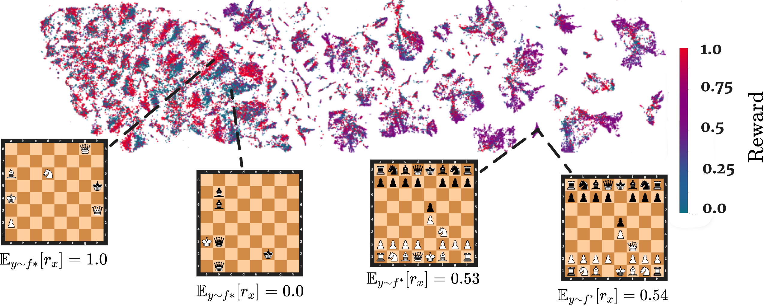
This image is a technical visualization, likely from a machine learning or reinforcement learning research paper, illustrating a latent space mapping of chess positions. It utilizes a dimensionality reduction technique (such as t-SNE or UMAP) to project high-dimensional chess states into a 2D plane, colored by a "Reward" metric.
---
## 2. Component Isolation
### Region A: Main Scatter Plot (Top)
* **Type:** 2D Scatter Plot / Heatmap.
* **Content:** A dense collection of data points representing individual chess positions.
* **Spatial Distribution:** The points are clustered into various "islands" or groupings, suggesting that the model has learned to group similar chess positions together in its latent space.
* **Color Gradient:** The points are colored based on a continuous scale.
* **Red/Magenta:** High density of high-reward positions.
* **Blue/Teal:** High density of low-reward positions.
* **Purple:** Intermediate reward values.
### Region B: Legend (Right Side)
* **Location:** [x: ~90%, y: ~40%]
* **Title:** "Reward" (oriented vertically).
* **Scale Type:** Continuous color bar.
* **Markers:**
* **1.0:** Bright Red (Top)
* **0.75:** Magenta
* **0.5:** Purple (Middle)
* **0.25:** Dark Blue
* **0.0:** Teal/Cyan (Bottom)
### Region C: Callout Examples (Bottom)
Four specific chess board configurations are pulled from the main plot via dashed lines to show the relationship between board state and the calculated reward value ($\mathbb{E}_{y \sim f^*}[r_x]$).
---
## 3. Data Extraction: Callout Boards
| Board Index (Left to Right) | Reward Value ($\mathbb{E}_{y \sim f^*}[r_x]$) | Visual Color Correlation | Key Board Features |
| :--- | :--- | :--- | :--- |
| **Board 1** | **1.0** | Red (High) | Endgame state. White has a significant material advantage (Queen, Knight, Bishop, Pawn) against a lone Black King. |
| **Board 2** | **0.0** | Teal (Low) | Endgame state. Black has a significant material advantage (Two Queens, two Bishops) against a lone White King. |
| **Board 3** | **0.53** | Purple (Mid) | Opening/Midgame state. Standard development (e.g., Ruy Lopez or Italian Game variation). Symmetrical material. |
| **Board 4** | **0.54** | Purple (Mid) | Opening/Midgame state. Similar to Board 3, showing a standard development phase with balanced material. |
---
## 4. Mathematical Notation
The image contains the following LaTeX-style mathematical expression beneath each board:
$$\mathbb{E}_{y \sim f^*}[r_x]$$
* **$\mathbb{E}$**: Expected value operator.
* **$y \sim f^*$**: Indicates that $y$ is sampled from the optimal distribution or ground truth function $f^*$.
* **$r_x$**: The reward associated with state $x$.
* **Interpretation:** This represents the expected reward of a given chess position $x$ under an optimal policy or ground truth evaluator.
---
## 5. Trend Analysis and Observations
1. **Clustering by Game Phase:** The scatter plot shows distinct clusters. The callouts suggest that the large, dense cluster on the left contains endgame positions (extreme rewards of 0.0 or 1.0), while the smaller clusters on the right represent opening or midgame positions (neutral rewards around 0.5).
2. **Reward Polarity:** The visualization effectively separates "winning" positions (Red) from "losing" positions (Teal) for the perspective being evaluated (presumably White).
3. **Spatial Grounding Logic Check:**
* The dashed line from **Board 1 (Reward 1.0)** points to a bright **Red** region in the far-left cluster.
* The dashed line from **Board 2 (Reward 0.0)** points to a **Teal** region within the same far-left cluster.
* The dashed lines from **Boards 3 and 4 (Rewards ~0.5)** point to **Purple** clusters on the right side of the map.
* *Verification:* The colors of the target regions in the scatter plot match the legend values and the numerical labels provided under the boards.