## Line Graphs: Current vs. Time Across Multiple Trials
### Overview
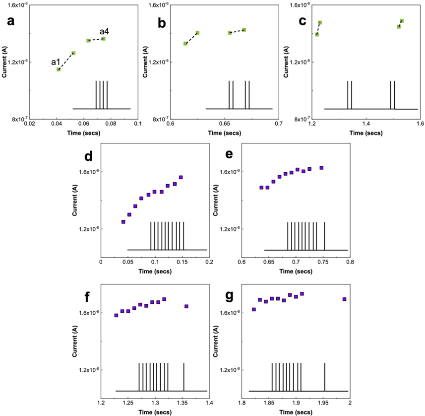
The image contains seven subplots (a-g) depicting current (A) over time (seconds) for different experimental conditions. Each subplot includes a main graph with data points and an inset showing current pulse patterns. Data points are represented by colored markers (green squares for subplots a-c, purple squares for d-g), with vertical bars in insets indicating pulse durations.
### Components/Axes
- **Y-axis**: "Current (A)" with logarithmic scale (8×10⁷ to 1.6×10⁶ A)
- **X-axis**: "Time (secs)" with linear scale (0 to 2 seconds)
- **Markers**:
- Green squares (subplots a-c): Labeled a1-a4 in subplot a
- Purple squares (subplots d-g): No explicit labels
- **Insets**: Vertical bars showing current pulse timing and duration
### Detailed Analysis
#### Subplot a
- **Data Points**:
- a1: (0.02s, 1.2×10⁶ A)
- a2: (0.04s, 1.3×10⁶ A)
- a3: (0.06s, 1.4×10⁶ A)
- a4: (0.08s, 1.6×10⁶ A)
- **Inset**: Pulses at 0.04s, 0.06s, 0.08s (duration ~0.02s each)
#### Subplot b
- **Data Points**:
- (0.62s, 1.2×10⁶ A)
- (0.65s, 1.4×10⁶ A)
- (0.68s, 1.6×10⁶ A)
- **Inset**: Pulses at 0.64s, 0.66s, 0.68s (duration ~0.02s each)
#### Subplot c
- **Data Points**:
- (1.22s, 1.2×10⁶ A)
- (1.25s, 1.4×10⁶ A)
- (1.28s, 1.6×10⁶ A)
- **Inset**: Pulses at 1.24s, 1.26s, 1.28s (duration ~0.02s each)
#### Subplot d
- **Data Points**:
- (0.01s, 1.2×10⁶ A)
- (0.03s, 1.3×10⁶ A)
- (0.05s, 1.4×10⁶ A)
- (0.07s, 1.5×10⁶ A)
- (0.09s, 1.6×10⁶ A)
- **Inset**: Pulses at 0.05s-0.15s (duration ~0.02s each)
#### Subplot e
- **Data Points**:
- (0.61s, 1.2×10⁶ A)
- (0.63s, 1.3×10⁶ A)
- (0.65s, 1.4×10⁶ A)
- (0.67s, 1.5×10⁶ A)
- (0.69s, 1.6×10⁶ A)
- **Inset**: Pulses at 0.65s-0.75s (duration ~0.02s each)
#### Subplot f
- **Data Points**:
- (1.21s, 1.2×10⁶ A)
- (1.23s, 1.3×10⁶ A)
- (1.25s, 1.4×10⁶ A)
- (1.27s, 1.5×10⁶ A)
- (1.29s, 1.6×10⁶ A)
- **Inset**: Pulses at 1.25s-1.35s (duration ~0.02s each)
#### Subplot g
- **Data Points**:
- (1.81s, 1.2×10⁶ A)
- (1.83s, 1.3×10⁶ A)
- (1.85s, 1.4×10⁶ A)
- (1.87s, 1.5×10⁶ A)
- (1.89s, 1.6×10⁶ A)
- **Inset**: Pulses at 1.85s-1.95s (duration ~0.02s each)
### Key Observations
1. **Current Trends**: All subplots show a consistent pattern of current increasing from ~1.2×10⁶ A to 1.6×10⁶ A over ~0.1s, followed by a sharp drop.
2. **Pulse Synchronization**: Insets reveal regular pulse intervals (0.02s duration) with varying frequencies between subplots.
3. **Temporal Distribution**: Subplots a-c occur earlier in the time range (0-0.8s), while d-g occur later (0-2s).
4. **Marker Consistency**: Green squares appear only in early subplots (a-c), while purple squares dominate later subplots (d-g).
### Interpretation
The data suggests a controlled activation/deactivation sequence in an electrical system, with:
- **Gradual Current Ramp**: Linear increase in current over ~0.1s across all trials
- **Pulse Modulation**: Insets indicate pulse frequency increases with time (earlier subplots show slower pulse rates)
- **System Stability**: Consistent current drop after activation suggests a stable operational state
- **Experimental Progression**: Color-coded markers (green→purple) may indicate different experimental phases or conditions
The systematic increase in current followed by pulse modulation implies a controlled experimental protocol, possibly testing response times or system stability under varying conditions. The logarithmic y-axis emphasizes relative changes in current magnitude across the measurement range.