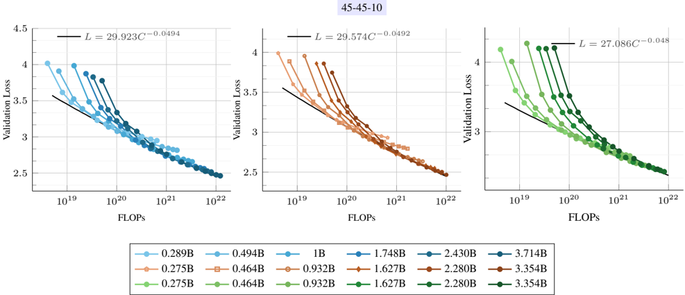
## Scatter Plot: Validation Loss vs. FLOPS for Different Model Sizes ### Overview The image presents three scatter plots arranged horizontally, each displaying the relationship between validation loss and FLOPS (Floating Point Operations Per Second) for different model sizes. Each plot contains multiple data series, each representing a specific model size, and a black line representing a power law fit. The plots share the same axes and general structure, but differ in the range of model sizes they depict. The title "45-45-10" is present at the top of the image. ### Components/Axes * **Title:** 45-45-10 (located at the top-center of the image) * **X-axis (Horizontal):** FLOPS (Floating Point Operations Per Second). The scale is logarithmic, ranging from approximately 10¹⁹ to 10²². * **Y-axis (Vertical):** Validation Loss. The scale is linear, ranging from 2.5 to 4.5. * **Data Series:** Each plot contains multiple data series, each represented by a different color and marker. Each series represents a different model size (in billions of parameters, denoted as 'B'). * **Power Law Fit:** Each plot includes a black line representing a power law fit to the data. The equation for the power law is displayed on each plot in the form L = aC^-b, where L is the validation loss, C is the FLOPS, and a and b are constants. * **Legend:** Located at the bottom of the image, the legend maps the colors and markers to the corresponding model sizes. ### Detailed Analysis **Plot 1 (Left):** * **Power Law Fit:** L = 29.923C^-0.0494 * **Data Series (from top-left to bottom-right):** * Light Blue: 0.289B. Starts at approximately (10¹⁹, 4.0) and decreases to (10²², 2.6). * Orange: 0.275B. Starts at approximately (10¹⁹, 3.9) and decreases to (10²², 2.6). * Green: 0.275B. Starts at approximately (10¹⁹, 3.8) and decreases to (10²², 2.5). * Blue: 0.494B. Starts at approximately (10¹⁹, 3.8) and decreases to (10²², 2.6). * Brown: 0.464B. Starts at approximately (10¹⁹, 3.7) and decreases to (10²², 2.6). * Dark Green: 0.464B. Starts at approximately (10¹⁹, 3.6) and decreases to (10²², 2.5). **Plot 2 (Center):** * **Power Law Fit:** L = 29.574C^-0.0492 * **Data Series (from top-left to bottom-right):** * Light Blue: 1B. Starts at approximately (10¹⁹, 4.0) and decreases to (10²², 2.6). * Orange: 0.932B. Starts at approximately (10¹⁹, 3.9) and decreases to (10²², 2.6). * Green: 0.932B. Starts at approximately (10¹⁹, 3.8) and decreases to (10²², 2.5). * Blue: 1.748B. Starts at approximately (10¹⁹, 3.7) and decreases to (10²², 2.6). * Brown: 1.627B. Starts at approximately (10¹⁹, 3.6) and decreases to (10²², 2.6). * Dark Green: 1.627B. Starts at approximately (10¹⁹, 3.5) and decreases to (10²², 2.5). **Plot 3 (Right):** * **Power Law Fit:** L = 27.086C^-0.048 * **Data Series (from top-left to bottom-right):** * Light Blue: 2.430B. Starts at approximately (10¹⁹, 4.2) and decreases to (10²², 2.6). * Orange: 2.280B. Starts at approximately (10¹⁹, 4.0) and decreases to (10²², 2.6). * Green: 2.280B. Starts at approximately (10¹⁹, 3.9) and decreases to (10²², 2.5). * Blue: 3.714B. Starts at approximately (10¹⁹, 3.8) and decreases to (10²², 2.6). * Brown: 3.354B. Starts at approximately (10¹⁹, 3.7) and decreases to (10²², 2.6). * Dark Green: 3.354B. Starts at approximately (10¹⁹, 3.6) and decreases to (10²², 2.5). ### Key Observations * **Inverse Relationship:** There is a clear inverse relationship between FLOPS and validation loss. As FLOPS increase, validation loss decreases. * **Power Law Behavior:** The power law fit suggests that the relationship between FLOPS and validation loss can be modeled by a power law function. * **Model Size Impact:** For a given FLOPS value, larger models (higher 'B' value) tend to have lower validation loss. * **Saturation:** The validation loss appears to saturate at higher FLOPS values, meaning that increasing FLOPS beyond a certain point yields diminishing returns in terms of reducing validation loss. * **Similar Trends:** The trends are very similar across the three plots, suggesting that the relationship between FLOPS and validation loss is consistent across different ranges of model sizes. * **Power Law Exponents:** The exponents in the power law fits are similar across the three plots (-0.0494, -0.0492, -0.048), suggesting a similar rate of decrease in validation loss with increasing FLOPS. ### Interpretation The plots demonstrate the relationship between computational effort (FLOPS) and model performance (validation loss) for different model sizes. The data suggests that increasing the computational effort invested in training a model leads to a reduction in validation loss, following a power law relationship. Furthermore, larger models tend to achieve lower validation loss for a given amount of computation. The saturation effect indicates that there are limits to the benefits of increasing FLOPS, and that other factors, such as model architecture or training data, may become more important at higher levels of computation. The consistency of the trends across the three plots suggests that these relationships are robust and generalizable across different model size ranges. The title "45-45-10" likely refers to specific experimental parameters or configurations used in the study.

\n ## Chart: Validation Loss vs. FLOPs for Different Model Sizes ### Overview The image presents three line charts, arranged horizontally, depicting the relationship between Validation Loss and FLOPs (Floating Point Operations) for various model sizes. Each chart represents a different scaling factor, indicated by the title "45-45-10". The charts aim to illustrate how model complexity (as measured by FLOPs) affects validation loss. ### Components/Axes * **X-axis:** FLOPs, ranging from approximately 10¹⁹ to 10²² (left chart), 10¹⁹ to 10²² (middle chart), and 10¹⁹ to 10²² (right chart). The scale is logarithmic. * **Y-axis:** Validation Loss, ranging from approximately 2.5 to 4.5. * **Title:** "45-45-10" appears above all three charts. * **Legend:** Located at the bottom of the image, containing labels for different model sizes: 0.289B, 0.499B, 1B, 1.748B, 2.430B, 3.714B, 0.275B, 0.464B, 0.932B, 1.627B, 2.280B, 3.354B. Each model size is associated with a specific color. * **Lines:** Each line represents a model size, with the color corresponding to the legend. Each line is labeled with an equation of the form "L = C₁C₂^-C₃", where C₁, C₂, and C₃ are numerical values. ### Detailed Analysis or Content Details **Chart 1 (Left):** * The black line (L = 29.923C^-0.0494) shows a steep downward slope, indicating a rapid decrease in validation loss as FLOPs increase. * The light blue line (0.289B) starts at approximately 4.0 and decreases to around 2.8 as FLOPs increase from 10¹⁹ to 10²². * The orange line (0.499B) starts at approximately 3.8 and decreases to around 2.7 as FLOPs increase. * The dark blue line (1B) starts at approximately 3.6 and decreases to around 2.6 as FLOPs increase. * The red line (1.748B) starts at approximately 3.4 and decreases to around 2.5 as FLOPs increase. * The green line (2.430B) starts at approximately 3.2 and decreases to around 2.4 as FLOPs increase. * The purple line (3.714B) starts at approximately 3.0 and decreases to around 2.3 as FLOPs increase. **Chart 2 (Middle):** * The black line (L = 29.574C^-0.0492) shows a steep downward slope. * The orange line (0.275B) starts at approximately 4.0 and decreases to around 2.7 as FLOPs increase. * The light blue line (0.464B) starts at approximately 3.8 and decreases to around 2.6 as FLOPs increase. * The green line (0.932B) starts at approximately 3.6 and decreases to around 2.5 as FLOPs increase. * The red line (1.627B) starts at approximately 3.4 and decreases to around 2.4 as FLOPs increase. * The dark blue line (2.280B) starts at approximately 3.2 and decreases to around 2.3 as FLOPs increase. * The purple line (3.354B) starts at approximately 3.0 and decreases to around 2.2 as FLOPs increase. **Chart 3 (Right):** * The black line (L = 27.086C^-0.048) shows a steep downward slope. * The green line (0.275B) starts at approximately 4.0 and decreases to around 2.7 as FLOPs increase. * The light blue line (0.464B) starts at approximately 3.8 and decreases to around 2.6 as FLOPs increase. * The orange line (0.932B) starts at approximately 3.6 and decreases to around 2.5 as FLOPs increase. * The red line (1.627B) starts at approximately 3.4 and decreases to around 2.4 as FLOPs increase. * The dark blue line (2.280B) starts at approximately 3.2 and decreases to around 2.3 as FLOPs increase. * The purple line (3.354B) starts at approximately 3.0 and decreases to around 2.2 as FLOPs increase. ### Key Observations * In all three charts, validation loss generally decreases as FLOPs increase, indicating that larger models (requiring more computation) tend to perform better. * The rate of decrease in validation loss appears to diminish as FLOPs increase, suggesting diminishing returns from increasing model size beyond a certain point. * The black lines in each chart represent a fitted curve, and the values of C₁, C₂, and C₃ change across the charts. * The lines are relatively close together, suggesting that the impact of model size on validation loss is consistent across the different scaling factors. ### Interpretation The charts demonstrate a clear trade-off between model complexity (FLOPs) and validation loss. Increasing model size generally leads to lower validation loss, but the improvement becomes less significant as the model grows larger. The fitted curves (black lines) provide a mathematical representation of this relationship, and the changing coefficients suggest that the optimal scaling factor may influence the specific form of this relationship. The consistent trend across the three charts suggests that this trade-off is a fundamental characteristic of the model architecture and training process. The "45-45-10" title likely refers to specific hyperparameters or experimental settings used during training, and further investigation would be needed to understand their influence on the observed results. The diminishing returns observed at higher FLOPs suggest that there may be a point of diminishing returns where increasing model size no longer provides a significant improvement in performance.

## [Chart Type]: Scaling Laws for Neural Language Models (Three-Panel Comparison) ### Overview The image displays three horizontally arranged scatter plots, each showing the relationship between computational cost (FLOPs) and model performance (Validation Loss) for neural language models of varying sizes. The plots are unified under the title "45-45-10" and share a common legend. Each plot contains multiple data series (representing different model parameter counts) and a fitted power-law curve. The overall trend demonstrates that validation loss decreases as computational resources (FLOPs) increase, following a predictable scaling law. ### Components/Axes * **Title:** "45-45-10" (centered at the top of the entire figure). * **Subplots:** Three distinct charts arranged left to right. * **X-Axis (All Plots):** Label: "FLOPs". Scale: Logarithmic, ranging from approximately 10¹⁹ to 10²². Major tick marks are at 10¹⁹, 10²⁰, 10²¹, and 10²². * **Y-Axis (All Plots):** Label: "Validation Loss". Scale: Linear, ranging from 2.5 to 4.5. Major tick marks are at 2.5, 3, 3.5, 4, and 4.5. * **Legend:** Positioned at the bottom center, spanning the width of all three plots. It contains 18 entries organized in three rows and six columns, mapping model parameter counts (in billions, denoted by "B") to specific colors and marker styles. * **Row 1 (Blue shades):** 0.289B, 0.494B, 1B, 1.748B, 2.430B, 3.714B * **Row 2 (Orange/Brown shades):** 0.275B, 0.464B, 0.932B, 1.627B, 2.280B, 3.354B * **Row 3 (Green shades):** 0.275B, 0.464B, 0.932B, 1.627B, 2.280B, 3.354B * **Fitted Curve Equations:** Each subplot contains a black line representing a power-law fit, with its equation displayed in the top-right corner of the plot area. * **Left Plot:** `L = 29.923C⁻⁰.⁰⁴⁹⁴` * **Middle Plot:** `L = 29.574C⁻⁰.⁰⁴⁹²` * **Right Plot:** `L = 27.086C⁻⁰.⁰⁴⁸` (Where `L` is Validation Loss and `C` is FLOPs). ### Detailed Analysis **Left Plot (Blue Series):** * **Data Series:** Six series in shades of blue, corresponding to the first row of the legend (0.289B to 3.714B parameters). * **Trend:** All six series show a clear downward slope, with validation loss decreasing as FLOPs increase. The series for larger models (darker blues) start at higher FLOPs and achieve lower final loss values. * **Key Data Points (Approximate):** * Smallest model (0.289B, lightest blue): Starts near (10¹⁹ FLOPs, 4.0 Loss), ends near (10²⁰ FLOPs, 3.2 Loss). * Largest model (3.714B, darkest blue): Starts near (10²⁰ FLOPs, 3.8 Loss), ends near (10²² FLOPs, 2.5 Loss). * **Fitted Curve:** The black line `L = 29.923C⁻⁰.⁰⁴⁹⁴` runs through the center of the data cloud, representing the average scaling trend. **Middle Plot (Orange/Brown Series):** * **Data Series:** Six series in shades of orange to brown, corresponding to the second row of the legend (0.275B to 3.354B parameters). * **Trend:** Identical downward trend to the left plot. The data points are tightly clustered around the fitted line. * **Key Data Points (Approximate):** * Smallest model (0.275B, lightest orange): Starts near (10¹⁹ FLOPs, 4.0 Loss), ends near (10²⁰ FLOPs, 3.2 Loss). * Largest model (3.354B, darkest brown): Starts near (10²⁰ FLOPs, 3.9 Loss), ends near (10²² FLOPs, 2.5 Loss). * **Fitted Curve:** The black line `L = 29.574C⁻⁰.⁰⁴⁹²` is nearly identical in shape and position to the left plot's curve. **Right Plot (Green Series):** * **Data Series:** Six series in shades of green, corresponding to the third row of the legend (0.275B to 3.354B parameters). * **Trend:** Consistent downward trend. The data points appear slightly more tightly grouped than in the other two plots. * **Key Data Points (Approximate):** * Smallest model (0.275B, lightest green): Starts near (10¹⁹ FLOPs, 4.2 Loss), ends near (10²⁰ FLOPs, 3.3 Loss). * Largest model (3.354B, darkest green): Starts near (10²⁰ FLOPs, 4.1 Loss), ends near (10²² FLOPs, 2.5 Loss). * **Fitted Curve:** The black line `L = 27.086C⁻⁰.⁰⁴⁸` has a slightly lower coefficient (27.086 vs. ~29.9) but a very similar exponent (~0.048 vs. ~0.049). ### Key Observations 1. **Consistent Scaling Law:** All three plots, despite representing different model families or training configurations (implied by the different color sets), exhibit the same fundamental power-law relationship between compute (FLOPs) and performance (Loss). The exponents of the fitted curves are remarkably similar (-0.0494, -0.0492, -0.048). 2. **Model Size Efficiency:** For a fixed FLOPs budget, larger models (darker markers) consistently achieve lower validation loss than smaller models. This is visible as the darker-colored points lying below the lighter-colored points at the same x-axis position. 3. **Diminishing Returns:** The curves flatten as FLOPs increase, indicating diminishing returns on investment. Doubling the compute yields a smaller absolute reduction in loss at the high-compute end (10²²) than at the low-compute end (10¹⁹). 4. **Data Alignment:** The empirical data points (colored markers) align very closely with the theoretical power-law fits (black lines), validating the scaling hypothesis across two orders of magnitude in model size and three orders of magnitude in compute. ### Interpretation This image provides strong empirical evidence for the "scaling laws" phenomenon in deep learning, specifically for language models. The data suggests that model performance (as measured by validation loss) is a smooth, predictable function of the computational resources used for training, largely independent of the specific model architecture details (as represented by the three different color families). The near-identical exponents across the three panels imply a universal scaling behavior. The primary difference lies in the coefficient (the `29.9`, `29.6`, `27.1` terms), which may reflect differences in data quality, training efficiency, or architectural innovations between the three model families being compared. The "45-45-10" title could refer to a specific data mixture ratio (e.g., 45% web text, 45% books, 10% code) used in these experiments. The practical implication is that one can forecast the performance of a larger model or the compute required for a target performance level with reasonable accuracy using these power-law fits. This enables efficient resource allocation in large-scale AI research. The plots also visually argue that simply increasing parameters without a corresponding increase in compute (moving vertically on the plot) is less effective than scaling both together along the established curve.

## Line Graphs: Validation Loss vs FLOPs (45-45-10) ### Overview Three side-by-side line graphs compare validation loss against computational resources (FLOPs) for different model sizes. Each graph shows a logarithmic relationship between FLOPs and validation loss, with distinct color-coded data series and fitted curves. ### Components/Axes - **X-axis (FLOPs)**: Logarithmic scale from 10¹⁹ to 10²². - **Y-axis (Validation Loss)**: Linear scale from 2.5 to 4.5. - **Legends**: - **Left Graph**: Blue (0.289B, 0.494B, 1B), Orange (0.275B, 0.464B, 0.932B), Green (0.275B, 0.464B, 0.932B). - **Middle Graph**: Blue (1B, 1.748B, 2.430B), Orange (0.932B, 1.627B, 2.280B), Green (0.932B, 1.627B, 2.280B). - **Right Graph**: Blue (2.430B, 3.714B), Orange (3.354B), Green (2.280B, 3.354B). - **Fitted Curves**: Black lines with equations (e.g., `L = 29.923C⁻⁰.⁰⁴⁹⁴` for the left graph). ### Detailed Analysis 1. **Left Graph (45-45-10)**: - **Blue Lines**: Slope downward steeply, with validation loss decreasing from ~4.0 to ~2.5 as FLOPs increase from 10¹⁹ to 10²². - **Orange Lines**: Similar trend but slightly higher validation loss at equivalent FLOPs. - **Green Lines**: Overlap with orange lines, suggesting identical performance for these sizes. 2. **Middle Graph (45-45-10)**: - **Blue Lines**: Validation loss decreases from ~4.0 to ~2.5, with steeper slopes than the left graph. - **Orange Lines**: Start at higher loss (~4.0) and decline more gradually. - **Green Lines**: Overlap with orange lines, indicating similar performance. 3. **Right Graph (45-45-10)**: - **Blue Lines**: Validation loss drops from ~4.0 to ~2.5, with the steepest slopes. - **Green Lines**: Start at ~4.0 and decline sharply, overlapping with blue lines at higher FLOPs. ### Key Observations - **Consistent Trend**: All graphs show validation loss decreasing as FLOPs increase, confirming the inverse relationship. - **Logarithmic Fit**: Equations (e.g., `L = 29.923C⁻⁰.⁰⁴⁹⁴`) indicate diminishing returns at higher FLOPs. - **Color Consistency**: Legend colors match line colors across graphs (e.g., blue = 0.289B in left, 1B in middle, 2.430B in right). - **Overlapping Lines**: Some sizes (e.g., 0.932B and 1.627B) show identical performance in certain graphs. ### Interpretation The data demonstrates that larger models (higher FLOPs) achieve lower validation loss, but with diminishing returns. The logarithmic fits suggest that computational efficiency plateaus beyond a certain threshold. Overlapping lines in some graphs imply that specific model sizes yield comparable performance, highlighting potential redundancy in resource allocation. The consistent trend across all graphs underscores the universal trade-off between computational cost and model accuracy.