## 3D Scatter Plot: Uniform Sampling on a Sphere
### Overview
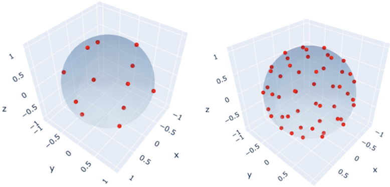
The image displays two side-by-side 3D scatter plots. Each plot visualizes a set of red data points distributed on the surface of a semi-transparent, light-blue sphere centered at the origin (0,0,0) within a 3D Cartesian coordinate system. The left plot shows a sparse distribution of points, while the right plot shows a much denser distribution. The visualization demonstrates the concept of sampling points uniformly on a spherical surface.
### Components/Axes
* **Chart Type:** 3D Scatter Plot (two instances).
* **Coordinate System:** 3D Cartesian.
* **Axes Labels:** All three axes are labeled:
* **X-axis:** Labeled "x". Ticks and values visible at -1, -0.5, 0, 0.5, 1.
* **Y-axis:** Labeled "y". Ticks and values visible at -1, -0.5, 0, 0.5, 1.
* **Z-axis:** Labeled "z". Ticks and values visible at -1, -0.5, 0, 0.5, 1.
* **Data Series:** A single series in each plot, represented by red circular markers.
* **Geometric Primitive:** A semi-transparent, light-blue sphere centered at (0,0,0) with a radius of 1 unit. The sphere's surface defines the locus for all data points.
* **Legend:** No legend is present in the image.
* **Titles:** No chart titles or subtitles are present.
### Detailed Analysis
**Left Plot (Sparse Sampling):**
* **Point Count:** Approximately 15 red data points are visible.
* **Spatial Distribution:** The points are scattered across the visible hemisphere of the sphere. They appear to be placed with intentional spacing, avoiding large clusters or gaps, suggesting an attempt at uniform or quasi-uniform distribution.
* **Trend Verification:** All points lie exactly on the surface of the sphere. There is no trend in the traditional sense (like a line sloping upward), as the data represents a static spatial distribution. The visual "trend" is one of even coverage.
**Right Plot (Dense Sampling):**
* **Point Count:** Approximately 50-60 red data points are visible.
* **Spatial Distribution:** The points are much more densely packed, covering the sphere's surface more thoroughly. The distribution still appears uniform, with no obvious clustering or patterning, indicating a higher-resolution sampling of the same spherical surface.
* **Trend Verification:** As with the left plot, all points are constrained to the sphere's surface. The increased density provides a clearer visual impression of the spherical shape.
**Common Elements:**
* **Viewing Angle:** Both plots share an identical isometric-like viewing perspective, looking down from a positive x, y, and z direction.
* **Axis Orientation:** The orientation of the x, y, and z axes is consistent between the two plots.
* **Sphere Representation:** The sphere is rendered with the same size, color, and transparency in both plots.
### Key Observations
1. **Constraint Adherence:** Every single data point in both plots lies precisely on the surface of the unit sphere. This is the primary and most critical observation.
2. **Density Contrast:** The fundamental difference between the two plots is the number of sample points, illustrating the concept of sampling density.
3. **Uniformity:** In both cases, the points do not form obvious lines, grids, or clusters. Their arrangement suggests a method designed to cover the spherical surface evenly, which is non-trivial in 3D space.
4. **Lack of Anomalies:** There are no outlier points floating inside or outside the sphere. The data is perfectly clean relative to the spherical constraint.
### Interpretation
This image is a technical visualization likely used to demonstrate or validate algorithms for **uniform sampling on a sphere**. Such algorithms are crucial in fields like computer graphics (for generating environment maps or particle systems), Monte Carlo integration, statistics, and physics simulations.
* **What the data suggests:** The plots show the output of a sampling algorithm at two different resolutions. The left plot could represent an initial or coarse sampling stage, while the right plot represents a refined or high-density sampling stage. The perfect adherence to the sphere's surface confirms the algorithm correctly enforces the geometric constraint.
* **How elements relate:** The sphere defines the problem domain (the unit sphere surface). The red points are the solution (the samples). The axes provide the necessary spatial reference frame to verify that the samples are correctly positioned in 3D space.
* **Notable patterns:** The key pattern is the *lack* of pattern—the points appear stochastically or quasi-randomly placed without regular structure, which is often the goal for uniform sampling to avoid aliasing artifacts. The side-by-side comparison effectively communicates the concept of increasing sample density to achieve better surface coverage.
**In summary, the image provides a clear, factual demonstration of point distributions on a spherical manifold, contrasting low-density and high-density uniform sampling results.**