\n
## Directed Graph Diagram: Network Flow with Theta Parameters
### Overview
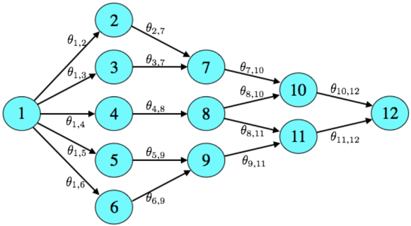
The image displays a directed acyclic graph (DAG) consisting of 12 nodes (circles) connected by directed edges (arrows). The graph flows from a single source node on the left to a single sink node on the right, with multiple branching and converging paths in between. Each edge is labeled with a parameter denoted by the Greek letter theta (θ) with a subscript indicating the source and destination nodes.
### Components/Axes
* **Nodes:** 12 circular nodes, each filled with a cyan color and containing a unique integer label from 1 to 12.
* **Edges:** Directed arrows connecting the nodes. Each edge has an associated label in the format `θ_{i,j}`, where `i` is the source node number and `j` is the destination node number.
* **Layout:** The graph is arranged in a layered, left-to-right flow.
* **Source Layer (Left):** Node 1.
* **First Branching Layer:** Nodes 2, 3, 4, 5, 6.
* **Intermediate Convergence Layer 1:** Nodes 7, 8, 9.
* **Intermediate Convergence Layer 2:** Nodes 10, 11.
* **Sink Layer (Right):** Node 12.
### Detailed Analysis
**Node and Edge Inventory:**
The graph's complete structure is defined by the following connections:
1. **From Node 1 (Source):**
* To Node 2: Edge labeled `θ_{1,2}`
* To Node 3: Edge labeled `θ_{1,3}`
* To Node 4: Edge labeled `θ_{1,4}`
* To Node 5: Edge labeled `θ_{1,5}`
* To Node 6: Edge labeled `θ_{1,6}`
2. **From Node 2:**
* To Node 7: Edge labeled `θ_{2,7}`
3. **From Node 3:**
* To Node 7: Edge labeled `θ_{3,7}`
4. **From Node 4:**
* To Node 8: Edge labeled `θ_{4,8}`
5. **From Node 5:**
* To Node 9: Edge labeled `θ_{5,9}`
6. **From Node 6:**
* To Node 9: Edge labeled `θ_{6,9}`
7. **From Node 7:**
* To Node 10: Edge labeled `θ_{7,10}`
8. **From Node 8:**
* To Node 10: Edge labeled `θ_{8,10}`
* To Node 11: Edge labeled `θ_{8,11}`
9. **From Node 9:**
* To Node 11: Edge labeled `θ_{9,11}`
10. **From Node 10:**
* To Node 12 (Sink): Edge labeled `θ_{10,12}`
11. **From Node 11:**
* To Node 12 (Sink): Edge labeled `θ_{11,12}`
**Pathways to Sink (Node 12):**
There are multiple distinct paths from the source (Node 1) to the sink (Node 12):
* Path A: 1 → 2 → 7 → 10 → 12
* Path B: 1 → 3 → 7 → 10 → 12
* Path C: 1 → 4 → 8 → 10 → 12
* Path D: 1 → 4 → 8 → 11 → 12
* Path E: 1 → 5 → 9 → 11 → 12
* Path F: 1 → 6 → 9 → 11 → 12
### Key Observations
1. **Structural Symmetry:** The graph exhibits a degree of symmetry. The top branch (via nodes 2 & 3) converges at node 7. The bottom branch (via nodes 5 & 6) converges at node 9. The middle branch (via node 4) splits at node 8 to feed both convergence points (nodes 10 and 11) of the final stage.
2. **Parameterization:** Every single connection in the network is explicitly parameterized by a unique `θ_{i,j}` value. This suggests the graph is a model where the relationships or transition weights between nodes are quantifiable and likely variable.
3. **Bottleneck Nodes:** Nodes 7, 8, 9, 10, and 11 act as convergence or distribution points. Node 8 is particularly notable as it is the only node that distributes its output to two different subsequent nodes (10 and 11).
### Interpretation
This diagram is a formal representation of a **network flow model, a dependency graph, or a probabilistic graphical model**. The theta parameters (`θ_{i,j}`) are the critical informational elements; they likely represent:
* **Weights or Capacities:** In a flow network, `θ` could be the capacity of the link from node `i` to node `j`.
* **Probabilities:** In a Markov chain or Bayesian network, `θ_{i,j}` could be the conditional probability of transitioning to state `j` given state `i`.
* **Costs or Strengths:** In an optimization or influence model, `θ` could represent the cost of traversal or the strength of the connection.
The structure itself reveals the system's logic: a single input (Node 1) is distributed across several parallel processes (Nodes 2-6), which are then aggregated and processed through intermediate stages (Nodes 7-9), further refined (Nodes 10-11), and finally consolidated into a single output (Node 12). The absence of cycles confirms it is an acyclic process, typical of computational pipelines, decision trees, or causal models. To make this model functional, one would need to assign numerical values to each of the 17 distinct theta parameters labeled in the graph.