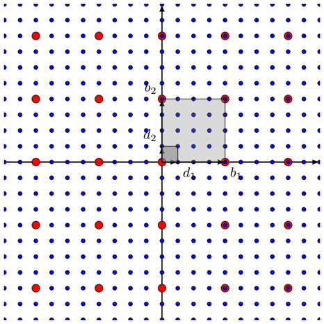
## Diagram: Grid with Labeled Regions and Data Points ### Overview The image depicts a 2D grid with labeled axes (x and y) and a shaded rectangular region. The grid contains two types of data points: red dots labeled "Data Points" and blue dots labeled "Reference Points." A legend in the top-right corner distinguishes these categories. The shaded region contains internal labels (d₁, d₂) and boundary labels (b₁, b₂), suggesting a focus on spatial relationships or measurements. --- ### Components/Axes - **Axes**: - Horizontal axis labeled "x" (rightward direction). - Vertical axis labeled "y" (upward direction). - **Legend**: - Located in the top-right corner. - Red dots = "Data Points." - Blue dots = "Reference Points." - **Shaded Region**: - Positioned in the upper-right quadrant of the grid. - Contains internal labels: - `d₁` (bottom-left corner of the shaded square). - `d₂` (top-left corner of the shaded square). - Boundary labels: - `b₁` (bottom-right corner of the shaded square). - `b₂` (top-right corner of the shaded square). --- ### Detailed Analysis - **Grid Structure**: - The grid is evenly spaced with blue dots forming a regular lattice. - Red dots are sparsely distributed, with some overlapping blue dots (e.g., at coordinates (2,3), (4,5), etc.). - **Shaded Region**: - The shaded square spans approximately 3 grid units horizontally and 2 grid units vertically. - Labels `d₁` and `d₂` likely represent distances or dimensions (e.g., width and height). - Labels `b₁` and `b₂` may denote boundary conditions or reference points for the shaded region. - **Data Point Distribution**: - Red "Data Points" are irregularly placed, with clusters near the shaded region (e.g., (3,4), (5,6)). - Blue "Reference Points" form a uniform grid, suggesting a baseline or control set. --- ### Key Observations 1. **Shaded Region Significance**: The shaded area highlights a specific subregion of interest, possibly for analysis or comparison. 2. **Data Point Density**: Red dots are concentrated near the shaded region, implying a potential relationship between the shaded area and the data points. 3. **Label Placement**: Labels `d₁`, `d₂`, `b₁`, and `b₂` are positioned at the corners of the shaded square, suggesting geometric or spatial measurements. 4. **Legend Consistency**: Red and blue dots align with their legend labels, confirming accurate categorization. --- ### Interpretation - **Purpose of the Diagram**: The image likely represents a spatial analysis framework, where the shaded region defines a target area for studying the distribution of "Data Points" relative to "Reference Points." - **Spatial Relationships**: The proximity of red dots to the shaded region may indicate a correlation between the shaded area and the observed data. For example, `d₁` and `d₂` could represent thresholds or critical dimensions influencing the data. - **Anomalies**: The overlap of red and blue dots at specific coordinates (e.g., (2,3)) might suggest overlapping categories or measurement errors. - **Uncertainty**: Without numerical values for `d₁`, `d₂`, `b₁`, or `b₂`, their exact significance remains ambiguous. However, their placement implies they are critical to defining the shaded region's properties. --- ### Conclusion This diagram serves as a spatial model for analyzing the distribution of data points within a defined region. The shaded area and its labels (`d₁`, `d₂`, `b₁`, `b₂`) are central to interpreting the relationship between the "Data Points" and "Reference Points." Further context (e.g., axis units, legend definitions) would enhance clarity.