# Technical Document Extraction: ArXiv Data Plot
## 1. Component Isolation
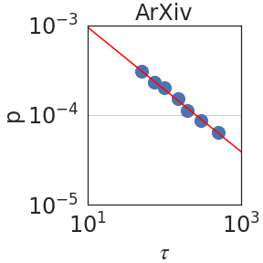
* **Header:** Contains the title "ArXiv".
* **Main Chart Area:** A log-log scatter plot with a superimposed linear regression line.
* **Axes:**
* **Y-axis (Vertical):** Labeled "$p$", representing a probability or density value.
* **X-axis (Horizontal):** Labeled "$\tau$", representing a time-scale or interval.
## 2. Axis and Scale Information
The chart utilizes a logarithmic scale (log-log) for both axes.
* **Y-axis ($p$):**
* **Range:** $10^{-5}$ to $10^{-3}$.
* **Major Markers:** $10^{-5}$, $10^{-4}$, $10^{-3}$.
* **Gridlines:** A faint horizontal gridline is present at the $10^{-4}$ mark.
* **X-axis ($\tau$):**
* **Range:** $10^{1}$ (10) to $10^{3}$ (1000).
* **Major Markers:** $10^{1}$, $10^{3}$.
* **Note:** The midpoint between $10^1$ and $10^3$ on a log scale is $10^2$ (100), which is where the data points are clustered.
## 3. Data Series Analysis
### Series 1: Observed Data (Blue Circles)
* **Visual Trend:** The data points follow a strict downward linear slope on the log-log scale, indicating a power-law relationship ($p \propto \tau^{-\alpha}$).
* **Spatial Grounding:** There are 7 distinct blue circular data points.
* **Estimated Data Points:**
1. $\tau \approx 50, p \approx 3 \times 10^{-4}$
2. $\tau \approx 70, p \approx 2.5 \times 10^{-4}$
3. $\tau \approx 100, p \approx 2 \times 10^{-4}$
4. $\tau \approx 150, p \approx 1.5 \times 10^{-4}$
5. $\tau \approx 200, p \approx 1 \times 10^{-4}$
6. $\tau \approx 300, p \approx 8 \times 10^{-5}$
7. $\tau \approx 500, p \approx 6 \times 10^{-5}$
### Series 2: Fit Line (Red Solid Line)
* **Visual Trend:** A solid red line slopes downward from the top-left toward the bottom-right.
* **Trend Verification:** The line acts as a "best fit" for the blue data points. It originates at $(\tau=10, p=10^{-3})$ and terminates near $(\tau=1000, p \approx 4 \times 10^{-5})$.
* **Slope Observation:** Since the line drops roughly 1.4 orders of magnitude over 2 orders of magnitude on the x-axis, the power-law exponent $\alpha$ is approximately $0.7$.
## 4. Summary of Information
| Feature | Description |
| :--- | :--- |
| **Dataset Name** | ArXiv |
| **Plot Type** | Log-Log Scatter with Linear Fit |
| **X-Axis Label** | $\tau$ (Tau) |
| **Y-Axis Label** | $p$ |
| **Relationship** | Inverse Power Law |
| **Data Range ($\tau$)** | $\sim 50$ to $\sim 500$ |
| **Data Range ($p$)** | $\sim 3 \times 10^{-4}$ to $\sim 6 \times 10^{-5}$ |
**Conclusion:** The image illustrates a statistical distribution from ArXiv data where the variable $p$ decreases as $\tau$ increases, following a power-law decay. The alignment of the blue points with the red line suggests a high degree of correlation for the model in the observed range.