## Line Graph: Model Accuracy vs. Compute (exaFLOP)
### Overview
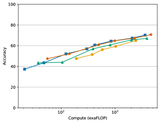
The image depicts a line graph comparing the accuracy of four computational models (A, B, C, D) across varying levels of compute power (exaFLOP). Accuracy is plotted on a linear y-axis (0–100%), while compute power is plotted on a logarithmic x-axis (10² to 10⁴ exaFLOP). All models show upward trends, with accuracy increasing as compute power grows.
### Components/Axes
- **Y-Axis (Accuracy)**: Labeled "Accuracy" with ticks at 0, 20, 40, 60, 80, 100.
- **X-Axis (Compute)**: Labeled "Compute (exaFLOP)" with logarithmic ticks at 10², 10³, and 10⁴.
- **Legend**: Located in the top-right corner, associating:
- Blue squares: Model A
- Red stars: Model B
- Green triangles: Model C
- Orange circles: Model D
### Detailed Analysis
1. **Model A (Blue Squares)**:
- Starts at ~40% accuracy at 10² exaFLOP.
- Rises steadily to ~70% at 10³ exaFLOP.
- Reaches ~75% at 10⁴ exaFLOP.
- **Trend**: Consistent linear growth with the steepest slope.
2. **Model B (Red Stars)**:
- Begins at ~45% accuracy at 10² exaFLOP.
- Accelerates to ~65% at 10³ exaFLOP.
- Peaks at ~72% at 10⁴ exaFLOP.
- **Trend**: Slightly concave upward, with faster gains at higher compute levels.
3. **Model C (Green Triangles)**:
- Starts at ~42% accuracy at 10² exaFLOP.
- Gains ~18% to reach ~60% at 10³ exaFLOP.
- Ends at ~68% at 10⁴ exaFLOP.
- **Trend**: Gradual, near-linear improvement.
4. **Model D (Orange Circles)**:
- Begins at ~40% accuracy at 10² exaFLOP.
- Increases to ~55% at 10³ exaFLOP.
- Reaches ~65% at 10⁴ exaFLOP.
- **Trend**: Slowest growth, with diminishing returns at higher compute levels.
### Key Observations
- All models improve accuracy with increased compute power, but efficiency varies.
- **Model A** and **Model B** achieve the highest accuracy, outperforming others by ~5–10% at 10⁴ exaFLOP.
- **Model D** lags behind, gaining only ~25% accuracy across the compute range.
- The logarithmic x-axis emphasizes that even modest compute increases (e.g., 10² to 10³) yield significant accuracy gains.
### Interpretation
The data suggests that computational efficiency and architectural design (Model A/B) are critical for maximizing accuracy. While all models benefit from increased compute, the diminishing returns for Model D imply potential limitations in scalability or optimization. The steepest gains for Models A and B highlight their superior resource utilization, making them preferable for high-stakes applications. The logarithmic scale underscores the exponential cost-benefit tradeoff: doubling compute power (e.g., 10³ to 10⁴ exaFLOP) yields smaller relative accuracy improvements, suggesting diminishing returns at extreme scales.