## Scatter Plot Matrix: Token Embeddings in Principal Component Space
### Overview
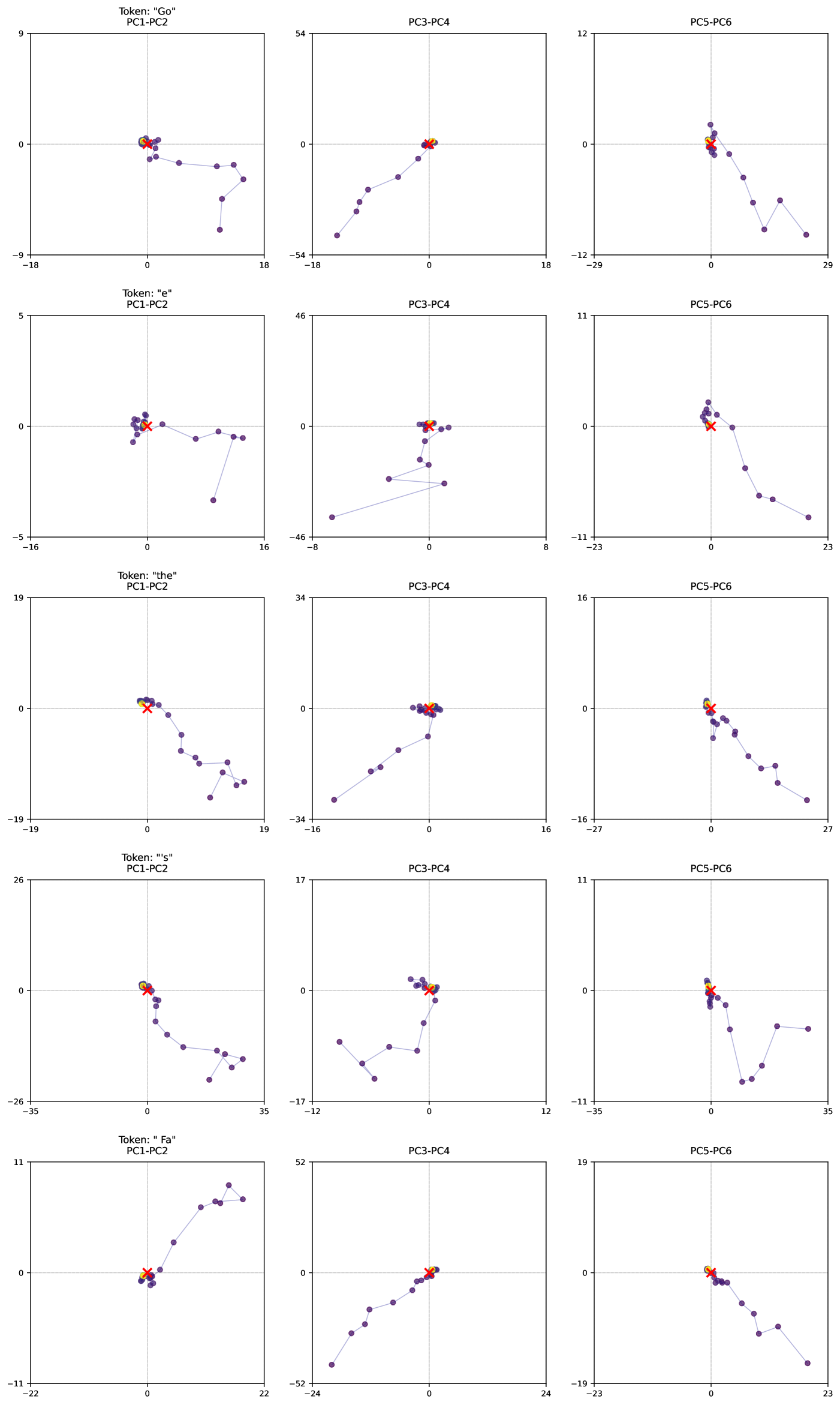
The image presents a matrix of scatter plots, visualizing the embeddings of five different tokens ("Go", "e", "the", "s", "Fa") in reduced dimensional spaces defined by principal components (PCs). Each row corresponds to a token, and each column represents a different pair of principal components (PC1-PC2, PC3-PC4, PC5-PC6). The plots show the trajectory of the token's embedding over time, with each point representing the embedding at a specific time step. A red 'X' marks the final embedding position.
### Components/Axes
Each scatter plot has the following components:
* **Title:** Indicates the token and the principal components being visualized (e.g., "Token: 'Go' PC1-PC2").
* **X-axis:** Represents the first principal component in the pair (e.g., PC1, PC3, PC5).
* **Y-axis:** Represents the second principal component in the pair (e.g., PC2, PC4, PC6).
* **Data Points:** Blue/purple dots connected by a light gray line, showing the trajectory of the token's embedding.
* **Final Embedding:** A red 'X' marks the final position of the token's embedding.
* **Axis Scales:** The scales vary across plots, but each axis is centered at zero. The ranges are approximately:
* PC1-PC2: -35 to 35
* PC3-PC4: -54 to 54
* PC5-PC6: -29 to 35
### Detailed Analysis
Each row represents a token, and each column represents a PC pair.
**Row 1: Token "Go"**
* **PC1-PC2:** The trajectory starts near the origin (0,0), moves slightly up and to the left, then loops down and to the right, ending near (10, -5).
* **PC3-PC4:** The trajectory starts near the origin, moves down and to the left, then curves back towards the origin, ending near (0,0).
* **PC5-PC6:** The trajectory starts near the origin, moves down and to the right, then loops back towards the origin, ending near (0,0).
**Row 2: Token "e"**
* **PC1-PC2:** The trajectory starts near the origin, moves slightly to the right, then loops back towards the origin, ending near (0,0).
* **PC3-PC4:** The trajectory starts near the origin, moves down and to the left, then loops back towards the origin, ending near (0,0).
* **PC5-PC6:** The trajectory starts near the origin, moves slightly to the right, then loops back towards the origin, ending near (0,0).
**Row 3: Token "the"**
* **PC1-PC2:** The trajectory starts near the origin, moves down and to the right, then loops back towards the origin, ending near (0,0).
* **PC3-PC4:** The trajectory starts near the origin, moves down and to the left, then loops back towards the origin, ending near (0,0).
* **PC5-PC6:** The trajectory starts near the origin, moves slightly to the right, then loops back towards the origin, ending near (0,0).
**Row 4: Token "s"**
* **PC1-PC2:** The trajectory starts near the origin, moves down and to the right, then loops back towards the origin, ending near (0,0).
* **PC3-PC4:** The trajectory starts near the origin, moves down and to the left, then loops back towards the origin, ending near (0,0).
* **PC5-PC6:** The trajectory starts near the origin, moves slightly to the right, then loops back towards the origin, ending near (0,0).
**Row 5: Token "Fa"**
* **PC1-PC2:** The trajectory starts near the origin, moves up and to the right, then loops back towards the origin, ending near (0,0).
* **PC3-PC4:** The trajectory starts near the origin, moves down and to the left, then loops back towards the origin, ending near (0,0).
* **PC5-PC6:** The trajectory starts near the origin, moves slightly to the right, then loops back towards the origin, ending near (0,0).
### Key Observations
* The trajectories for all tokens tend to start near the origin (0,0) in all PC pairs.
* The final embedding positions (red 'X') are also generally close to the origin.
* The PC3-PC4 plots show the most significant movement away from the origin for most tokens.
* The PC5-PC6 plots show the least movement away from the origin.
* The scales of the axes vary significantly between the PC pairs, suggesting different variances in the data along these principal components.
### Interpretation
The plots visualize how the embeddings of different tokens evolve over time in the reduced dimensional spaces defined by principal components. The fact that the trajectories start and end near the origin suggests that the tokens' embeddings tend to converge towards a central point in the high-dimensional space. The different scales of the axes indicate that the principal components capture varying amounts of variance in the data. PC3 and PC4 seem to capture more significant variations in the token embeddings compared to PC5 and PC6. The specific shapes of the trajectories might reflect the dynamic changes in the token's meaning or usage context over time. The differences in trajectories between tokens suggest that each token has a unique pattern of variation in the principal component space.