## Scatter Plot Matrix: Principal Component Analysis (PCA) for Tokens
### Overview
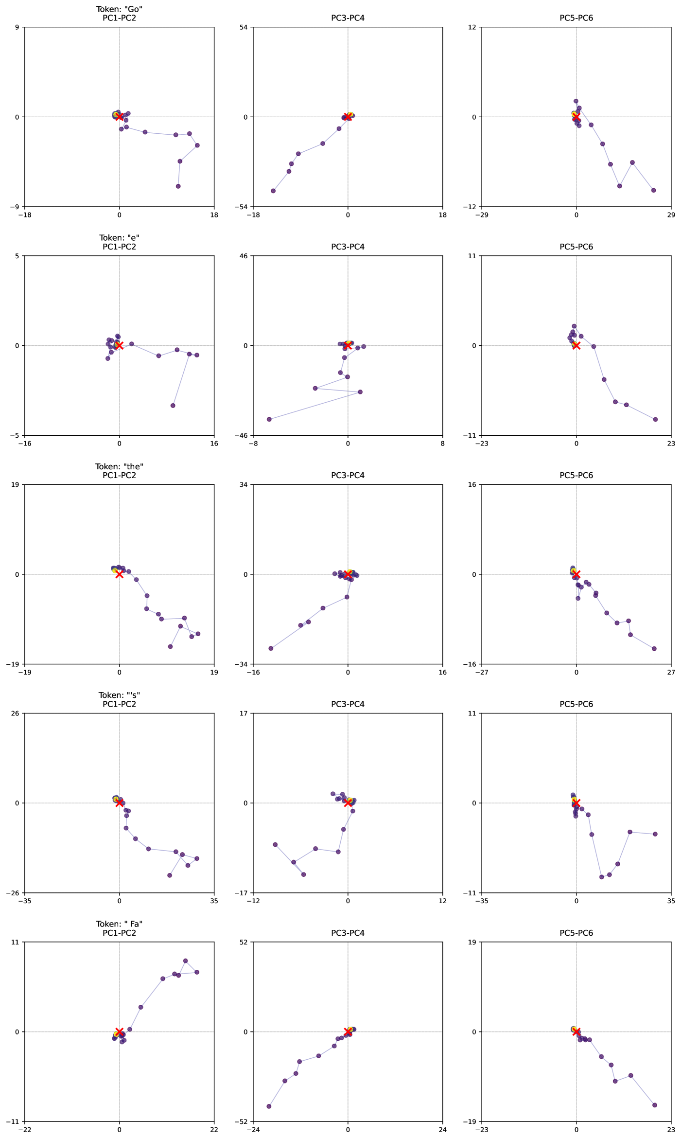
The image presents a scatter plot matrix visualizing the results of a Principal Component Analysis (PCA) performed on five different tokens: "Go", "e", "The", "!", and "Fa". Each token is represented by a different color, and the plots show the relationships between different principal components (PC1-PC6). There are 3 columns of plots, each showing a different pair of principal components.
### Components/Axes
The matrix consists of 15 individual scatter plots arranged in a 5x3 grid. Each plot displays two principal components as axes. The axes are labeled as follows:
* **Column 1:** PC1-PC2
* **Column 2:** PC3-PC4
* **Column 3:** PC5-PC6
Each plot has axes ranging from approximately -54 to 54 (PC1-PC2, PC3-PC4) and -35 to 35 (PC5-PC6). The tokens are represented by the following colors:
* "Go": Dark Red
* "e": Light Blue
* "The": Dark Blue
* "!": Dark Green
* "Fa": Dark Orange
### Detailed Analysis or Content Details
**Row 1: Token "Go"**
* **PC1-PC2:** The data points for "Go" (dark red) form a generally downward sloping curve. Approximate data points: (-16, -1.5), (-10, -3), (-5, -5), (0, -6), (5, -5), (10, -3), (16, -1.5).
* **PC3-PC4:** The "Go" data points (dark red) show a roughly linear, upward trend. Approximate data points: (-18, -54), (-8, -46), (0, -38), (8, -30), (18, -22).
* **PC5-PC6:** The "Go" data points (dark red) form a curved line, initially decreasing and then increasing. Approximate data points: (-29, -12), (-19, -10), (-9, -8), (0, -6), (9, -8), (19, -10), (29, -12).
**Row 2: Token "e"**
* **PC1-PC2:** The "e" data points (light blue) are scattered, with a slight upward trend. Approximate data points: (-16, -1), (-8, 0), (0, 1), (8, 2), (16, 3).
* **PC3-PC4:** The "e" data points (light blue) show a downward sloping curve. Approximate data points: (-18, 46), (-9, 38), (0, 30), (9, 22), (18, 14).
* **PC5-PC6:** The "e" data points (light blue) form a relatively straight line with a slight positive slope. Approximate data points: (-23, 11), (-11, 10), (1, 9), (13, 8), (23, 7).
**Row 3: Token "The"**
* **PC1-PC2:** The "The" data points (dark blue) show a curved line, initially decreasing and then increasing. Approximate data points: (-19, -19), (-9, -16), (0, -13), (9, -10), (19, -7).
* **PC3-PC4:** The "The" data points (dark blue) form a downward sloping curve. Approximate data points: (-16, 34), (-8, 28), (0, 22), (8, 16), (16, 10).
* **PC5-PC6:** The "The" data points (dark blue) show a curved line, initially decreasing and then increasing. Approximate data points: (-27, 16), (-13, 14), (1, 12), (15, 10), (27, 8).
**Row 4: Token "!"**
* **PC1-PC2:** The "!" data points (dark green) show a curved line, initially increasing and then decreasing. Approximate data points: (-26, 26), (-13, 30), (0, 32), (13, 30), (26, 26).
* **PC3-PC4:** The "!" data points (dark green) form a downward sloping curve. Approximate data points: (-12, 17), (-6, 14), (0, 11), (6, 8), (12, 5).
* **PC5-PC6:** The "!" data points (dark green) show a curved line, initially decreasing and then increasing. Approximate data points: (-35, 11), (-17, 10), (1, 9), (19, 10), (35, 11).
**Row 5: Token "Fa"**
* **PC1-PC2:** The "Fa" data points (dark orange) show a curved line, initially decreasing and then increasing. Approximate data points: (-22, 11), (-11, 8), (0, 5), (11, 2), (22, -1).
* **PC3-PC4:** The "Fa" data points (dark orange) show a generally upward sloping curve. Approximate data points: (-24, -52), (-12, -44), (0, -36), (12, -28), (24, -20).
* **PC5-PC6:** The "Fa" data points (dark orange) show a curved line, initially decreasing and then increasing. Approximate data points: (-23, 19), (-11, 16), (1, 13), (13, 10), (23, 7).
### Key Observations
* The tokens exhibit different distributions across the principal components, suggesting they are distinguishable based on these features.
* The "Go" token shows a clear downward trend in PC1-PC2, while "e" shows a slight upward trend.
* The "!" token has a more pronounced curved shape in PC1-PC2 compared to other tokens.
* The PC3-PC4 plots generally show downward trends for all tokens.
* The PC5-PC6 plots show more complex curved patterns for most tokens.
### Interpretation
This PCA plot matrix visualizes how different tokens are separated in a lower-dimensional space defined by the principal components. Each token's distribution reveals its unique characteristics based on the underlying data used for the PCA. The different trends observed in each plot suggest that the principal components capture different aspects of the tokens' variability. For example, PC1-PC2 might be capturing the overall "complexity" of the token, while PC3-PC4 might be related to its "frequency" or "position" within the data. The curved shapes observed in some plots indicate non-linear relationships between the original features and the principal components. This analysis could be used for token classification, clustering, or dimensionality reduction in natural language processing or other related fields. The differences in the distributions of the tokens across the principal components suggest that they are relatively distinct and can be effectively separated using PCA.