## Chart: Test Loss vs. Parameters ### Overview The image presents two line charts comparing the test loss of models with varying numbers of layers against the number of parameters. The left chart shows the relationship when parameters include embeddings, while the right chart excludes embeddings. The number of layers is represented by different colored lines. ### Components/Axes **Left Chart:** * **Title:** Parameters (with embedding) * **X-axis:** Parameters (with embedding), logarithmic scale from 10^6 to 10^9 * **Y-axis:** Test Loss, linear scale from 2 to 7 * **Legend (top-left):** * Dark Blue: 0 Layer * Purple: 1 Layer * Medium Purple: 2 Layers * Pink: 3 Layers * Light Orange: 6 Layers * Orange: > 6 Layers **Right Chart:** * **Title:** Parameters (non-embedding) * **X-axis:** Parameters (non-embedding), logarithmic scale from 10^3 to 10^9 * **Y-axis:** Test Loss, linear scale from 2 to 7 * **Legend (left):** * Purple: 1 Layer * Medium Purple: 2 Layers * Pink: 3 Layers * Light Orange: 6 Layers * Orange: > 6 Layers ### Detailed Analysis **Left Chart (with embedding):** * **0 Layer (Dark Blue):** Starts at approximately 6.8 test loss at 10^6 parameters, remains relatively flat around 6.0 test loss until 10^9 parameters. * **1 Layer (Purple):** Starts at approximately 7.0 test loss at 10^6 parameters, decreases to approximately 3.5 test loss at 10^9 parameters. * **2 Layers (Medium Purple):** Starts at approximately 6.0 test loss at 10^6 parameters, decreases to approximately 3.0 test loss at 10^9 parameters. * **3 Layers (Pink):** Starts at approximately 5.0 test loss at 10^6 parameters, decreases to approximately 2.7 test loss at 10^9 parameters. * **6 Layers (Light Orange):** Starts at approximately 4.5 test loss at 10^6 parameters, decreases to approximately 2.5 test loss at 10^9 parameters. * **> 6 Layers (Orange):** Starts at approximately 4.0 test loss at 10^6 parameters, decreases to approximately 2.3 test loss at 10^9 parameters. **Right Chart (non-embedding):** * **1 Layer (Purple):** Starts at approximately 6.5 test loss at 10^3 parameters, decreases to approximately 4.2 test loss at 10^9 parameters. * **2 Layers (Medium Purple):** Starts at approximately 6.0 test loss at 10^3 parameters, decreases to approximately 3.5 test loss at 10^9 parameters. * **3 Layers (Pink):** Starts at approximately 6.0 test loss at 10^3 parameters, decreases to approximately 3.0 test loss at 10^9 parameters. * **6 Layers (Light Orange):** Starts at approximately 5.5 test loss at 10^3 parameters, decreases to approximately 2.5 test loss at 10^9 parameters. * **> 6 Layers (Orange):** Starts at approximately 5.0 test loss at 10^3 parameters, decreases to approximately 2.3 test loss at 10^9 parameters. ### Key Observations * In both charts, increasing the number of parameters generally leads to a decrease in test loss. * The "0 Layer" model in the left chart (with embedding) shows minimal improvement in test loss as the number of parameters increases. * The right chart (non-embedding) shows a steeper initial decrease in test loss for all models as the number of parameters increases from 10^3 to 10^6, compared to the left chart. * The models with more layers (6 and >6) consistently achieve lower test loss compared to models with fewer layers (1, 2, and 3) in both charts. ### Interpretation The charts suggest that increasing the number of layers and parameters in a model generally improves its performance, as indicated by the decrease in test loss. The inclusion of embeddings appears to shift the parameter scale, requiring more parameters to achieve similar test loss reductions compared to models without embeddings. The "0 Layer" model's flat performance in the left chart indicates that simply increasing parameters without adding layers does not significantly improve performance. The steeper initial decrease in test loss in the right chart suggests that the initial impact of increasing parameters is more pronounced when embeddings are not included. The models with more layers consistently outperform those with fewer layers, highlighting the importance of model depth in achieving better results.

\n ## Chart: Test Loss vs. Parameters for Different Layer Depths ### Overview The image presents two line charts comparing the test loss of models with varying numbers of layers against the number of parameters. The left chart shows results for models *with embedding*, while the right chart shows results for models *without embedding*. Both charts use a logarithmic scale for the x-axis (Parameters). ### Components/Axes * **X-axis (Both Charts):** Parameters. The left chart's scale ranges from approximately 10⁶ to 10⁹. The right chart's scale ranges from approximately 10³ to 10⁹. * **Y-axis (Both Charts):** Test Loss. The scale ranges from approximately 2 to 7. * **Left Chart Legend (Top-Left):** * 0 Layer (Blue) * 1 Layer (Purple) * 2 Layers (Dark Red) * 3 Layers (Orange) * 6 Layers (Yellow) * > 6 Layers (Brown) * **Right Chart Legend (Top-Right):** * 1 Layer (Purple) * 2 Layers (Dark Red) * 3 Layers (Orange) * 6 Layers (Yellow) * > 6 Layers (Brown) ### Detailed Analysis or Content Details **Left Chart (With Embedding):** * **0 Layer (Blue):** Starts at approximately 6.8 and remains relatively flat, decreasing slightly to around 6.2 at 10⁹ parameters. * **1 Layer (Purple):** Starts at approximately 6.8 and decreases steadily to around 3.8 at 10⁹ parameters. * **2 Layers (Dark Red):** Starts at approximately 6.5 and decreases more rapidly than the 1-layer model, reaching around 3.2 at 10⁹ parameters. * **3 Layers (Orange):** Starts at approximately 6.2 and decreases rapidly, reaching around 2.8 at 10⁹ parameters. * **6 Layers (Yellow):** Starts at approximately 5.5 and decreases very rapidly, reaching around 2.4 at 10⁹ parameters. * **> 6 Layers (Brown):** Starts at approximately 5.2 and decreases most rapidly, reaching around 2.2 at 10⁹ parameters. **Right Chart (Non-Embedding):** * **1 Layer (Purple):** Starts at approximately 6.8 and decreases steadily to around 3.7 at 10⁹ parameters. * **2 Layers (Dark Red):** Starts at approximately 6.5 and decreases more rapidly than the 1-layer model, reaching around 3.1 at 10⁹ parameters. * **3 Layers (Orange):** Starts at approximately 6.2 and decreases rapidly, reaching around 2.7 at 10⁹ parameters. * **6 Layers (Yellow):** Starts at approximately 5.5 and decreases very rapidly, reaching around 2.3 at 10⁹ parameters. * **> 6 Layers (Brown):** Starts at approximately 5.2 and decreases most rapidly, reaching around 2.1 at 10⁹ parameters. ### Key Observations * In both charts, increasing the number of layers consistently reduces the test loss. * The rate of loss reduction appears to diminish as the number of parameters increases, especially for models with more layers. * The models with embedding (left chart) generally exhibit slightly higher test loss values compared to the models without embedding (right chart) for the same number of layers and parameters. * The 0-layer model (left chart) shows minimal improvement in test loss with increasing parameters, suggesting it is not benefiting from increased model capacity. ### Interpretation The data demonstrates a clear relationship between model complexity (number of layers) and performance (test loss). Increasing the number of layers generally leads to lower test loss, indicating improved model accuracy. However, the diminishing returns observed at higher parameter counts suggest that there is a point of saturation where adding more layers does not significantly improve performance. The difference between the "with embedding" and "non-embedding" models suggests that embedding may provide a slight advantage in terms of test loss, but this advantage is not substantial. The 0-layer model's lack of improvement highlights the importance of model capacity for learning complex patterns. The logarithmic scale on the x-axis emphasizes the impact of increasing parameters, particularly at lower values. The charts provide valuable insights into the trade-offs between model complexity, parameter count, and performance, which can inform model design and optimization strategies. The consistent downward trend for all layer counts suggests that increasing model size is generally beneficial, but careful consideration should be given to the point of diminishing returns and the potential benefits of embedding techniques.

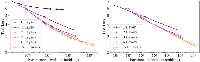
## Dual Line Charts: Model Scaling vs. Test Loss ### Overview The image displays two side-by-side line charts analyzing the relationship between model size (measured in parameters) and test loss. The left chart uses total parameters including embeddings, while the right chart uses non-embedding parameters. Both charts show that as the number of parameters increases, test loss decreases, with deeper models (more layers) achieving lower loss for a given parameter count. ### Components/Axes **Common Elements:** * **Chart Type:** Two line charts with logarithmic x-axes. * **Y-Axis (Both Charts):** Label: "Test Loss". Scale: Linear, ranging from 2 to 7. * **Legend (Both Charts):** Located in the top-left corner of each plot area. Contains colored lines and labels for different model depths. * **Line Colors & Labels:** * Dark Blue: "0 Layer" (Left chart only) * Purple: "1 Layer" * Magenta: "2 Layers" * Red: "3 Layers" * Orange: "6 Layers" * Yellow: "> 6 Layers" **Left Chart Specifics:** * **Title/Context:** Implicitly compares models using total parameter count. * **X-Axis:** Label: "Parameters (with embedding)". Scale: Logarithmic, with major ticks at 10⁶, 10⁷, 10⁸, 10⁹. **Right Chart Specifics:** * **Title/Context:** Implicitly compares models using non-embedding parameter count. * **X-Axis:** Label: "Parameters (non-embedding)". Scale: Logarithmic, with major ticks at 10³, 10⁴, 10⁵, 10⁶, 10⁷, 10⁸, 10⁹. ### Detailed Analysis **Left Chart (Parameters with embedding):** * **0 Layer (Dark Blue):** Starts at ~7.0 loss for ~10⁵ parameters. Shows a shallow, nearly flat decline, ending at ~6.0 loss for ~10⁸ parameters. This line is the highest (worst loss) and has the shallowest slope. * **1 Layer (Purple):** Starts near 7.0 loss for ~10⁵ parameters. Slopes downward more steeply than the 0-layer line, ending at ~3.5 loss for ~10⁹ parameters. * **2 Layers (Magenta):** Follows a path below the 1-layer line. Starts near 7.0 loss, ends at ~2.8 loss for ~10⁹ parameters. * **3 Layers (Red):** Follows a path below the 2-layer line. Ends at ~2.6 loss for ~10⁹ parameters. * **6 Layers (Orange):** Follows a path below the 3-layer line. Ends at ~2.5 loss for ~10⁹ parameters. * **> 6 Layers (Yellow):** Follows the lowest path, nearly overlapping with the 6-layer line at the high-parameter end. Ends at ~2.4 loss for ~10⁹ parameters. * **Trend:** All lines show a clear inverse relationship. For a fixed parameter count (e.g., 10⁸), test loss decreases as the number of layers increases (0 Layer > 1 Layer > 2 Layers...). **Right Chart (Parameters non-embedding):** * **1 Layer (Purple):** Starts at ~6.5 loss for ~10³ parameters. Slopes downward, ending at ~3.5 loss for ~10⁸ parameters. * **2 Layers (Magenta):** Follows a path below the 1-layer line. Ends at ~2.8 loss for ~10⁹ parameters. * **3 Layers (Red):** Follows a path below the 2-layer line. Ends at ~2.6 loss for ~10⁹ parameters. * **6 Layers (Orange):** Follows a path below the 3-layer line. Ends at ~2.5 loss for ~10⁹ parameters. * **> 6 Layers (Yellow):** Follows the lowest path, nearly overlapping with the 6-layer line. Ends at ~2.4 loss for ~10⁹ parameters. * **Trend:** Similar inverse relationship. The lines for 2+ layers are tightly clustered, especially at higher parameter counts, suggesting diminishing returns from adding layers beyond a certain point when controlling for non-embedding parameters. ### Key Observations 1. **The "0 Layer" Baseline:** The 0-layer model (left chart only) performs significantly worse and scales poorly compared to any model with at least one layer. 2. **Layer Efficiency:** For the same total parameter budget (left chart), adding layers consistently improves performance (lowers loss). The gap between lines is most pronounced at lower parameter counts. 3. **Convergence at Scale:** In both charts, the performance lines for models with 3, 6, and >6 layers converge as parameter count increases towards 10⁹. This suggests that at very large scales, the advantage of extreme depth diminishes. 4. **Parameter Accounting:** The right chart shifts all curves to the left (lower parameter values) because it excludes embedding parameters, which can be a large portion of the total in language models. This reveals the scaling behavior of the core transformer layers. ### Interpretation These charts demonstrate fundamental scaling laws for neural language models. The data suggests: * **Depth is Crucial:** Moving from a 0-layer to a 1-layer model provides a massive performance leap. Further depth continues to yield benefits, but with diminishing returns. * **Scaling Efficiency:** The near-linear decline on a log-linear plot (log x, linear y) indicates a power-law relationship between parameters and loss. This is a hallmark of efficient scaling. * **Architectural Insight:** The convergence of deeper models at high parameter counts implies that given enough capacity, models of varying depths can achieve similar final performance. The choice between a very deep vs. a moderately deep but wider model may then depend on other factors like inference cost or training stability. * **Practical Implication:** For a fixed compute budget (which correlates with parameters), allocating resources to increase depth (up to a point) is more beneficial than creating a shallow, massive model. The charts provide a visual guide for making such architectural trade-offs.

## Line Graphs: Test Loss vs. Parameters (Embedding vs. Non-Embedding) ### Overview The image contains two side-by-side line graphs comparing test loss performance across different neural network layer configurations. The left graph shows results for models with embedding layers, while the right graph shows results for models without embedding layers. Both graphs plot test loss (y-axis) against the number of parameters (x-axis, logarithmic scale). ### Components/Axes **Left Graph (With Embedding):** - **X-axis**: Parameters (with embedding) [10⁶ to 10⁹] - **Y-axis**: Test Loss [2 to 7] - **Legend**: - 0 Layer (dark blue) - 1 Layer (purple) - 2 Layers (pink) - 3 Layers (red) - 6 Layers (orange) - >6 Layers (yellow) **Right Graph (Non-Embedding):** - **X-axis**: Parameters (non-embedding) [10³ to 10⁹] - **Y-axis**: Test Loss [2 to 7] - **Legend**: - 1 Layer (dark blue) - 2 Layers (purple) - 3 Layers (pink) - 6 Layers (orange) - >6 Layers (yellow) ### Detailed Analysis **Left Graph Trends:** - 0 Layer (dark blue): Flat line at ~6.8 test loss (no parameter dependence) - 1 Layer (purple): Steep decline from ~6.5 to ~3.2 as parameters increase - 2 Layers (pink): Gradual decline from ~6.0 to ~2.8 - 3 Layers (red): Moderate decline from ~5.5 to ~2.5 - 6 Layers (orange): Steady decline from ~5.0 to ~2.2 - >6 Layers (yellow): Slight decline from ~4.8 to ~2.1 **Right Graph Trends:** - 1 Layer (dark blue): Sharp decline from ~6.5 to ~3.0 - 2 Layers (purple): Steep decline from ~6.0 to ~2.8 - 3 Layers (pink): Gradual decline from ~5.5 to ~2.5 - 6 Layers (orange): Steady decline from ~5.0 to ~2.2 - >6 Layers (yellow): Slight decline from ~4.8 to ~2.1 ### Key Observations 1. **Embedding vs. Non-Embedding**: - The non-embedding graph starts at 1 Layer (no 0 Layer baseline) - Both graphs show similar performance trends for ≥1 layers - Embedding models require significantly more parameters (10⁶ vs. 10³ baseline) 2. **Layer Complexity**: - Adding layers reduces test loss, but diminishing returns occur after 6 layers - >6 Layers show minimal improvement despite increased parameter count 3. **Parameter Efficiency**: - Non-embedding models achieve similar performance with 100-1000x fewer parameters - Embedding models require ~10⁶ parameters to reach ~2.2 test loss vs. ~10⁵ parameters for non-embedding ### Interpretation The data demonstrates that: - **Embedding layers** significantly increase parameter requirements but enable more complex architectures - **Layer count** has a logarithmic relationship with test loss improvement - **Diminishing returns** occur after 6 layers in both configurations - **Non-embedding models** achieve comparable performance with fewer parameters, suggesting embeddings may introduce unnecessary complexity for simpler tasks The flat 0 Layer line in the embedding graph indicates a potential baseline model (e.g., a simple classifier) that doesn't benefit from additional parameters. The convergence of >6 Layers lines suggests architectural saturation points where adding more layers provides minimal benefit.