## Heatmap: Reynolds Stress Anisotropy Components
### Overview
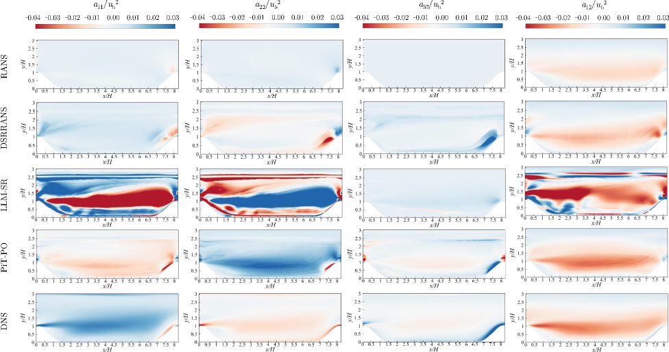
The image presents a series of heatmaps visualizing the Reynolds stress anisotropy components (a11/ub^2, a22/ub^2, a33/ub^2, a12/ub^2) for different turbulence models (RANS, DSRRANS, LLM-SR, PIT-PO, DNS) in a channel flow with a varying bottom topography. The x-axis represents the streamwise direction (x/H), and the y-axis represents the vertical direction (y/H). The color scale indicates the magnitude of the anisotropy components, with blue representing negative values and red representing positive values.
### Components/Axes
* **Rows (Turbulence Models):**
* RANS (Reynolds-Averaged Navier-Stokes)
* DSRRANS (Data-Driven Scale Resolving RANS)
* LLM-SR (Likelihood Maximization Model - Scale Resolving)
* PIT-PO (Pressure Implicit with Turbulence - Partially Optimized)
* DNS (Direct Numerical Simulation)
* **Columns (Anisotropy Components):**
* Column 1: a11/ub^2
* Column 2: a22/ub^2
* Column 3: a33/ub^2
* Column 4: a12/ub^2
* **X-axis:** x/H (Streamwise direction), ranging from approximately 0 to 8, with tick marks at intervals of 0.5.
* **Y-axis:** y/H (Vertical direction), ranging from 0 to 3, with tick marks at intervals of 0.5.
* **Color Scale:** Ranges from approximately -0.04 (dark blue) to 0.03 (dark red).
### Detailed Analysis
**Row 1: RANS**
* **a11/ub^2:** Predominantly light blue, indicating slightly negative values.
* **a22/ub^2:** Predominantly light blue, indicating slightly negative values.
* **a33/ub^2:** Predominantly light blue, indicating slightly negative values.
* **a12/ub^2:** Predominantly light blue, indicating slightly negative values.
**Row 2: DSRRANS**
* **a11/ub^2:** Mostly light blue, with a slight increase in magnitude near the bottom topography.
* **a22/ub^2:** Mostly light blue, with a slight increase in magnitude near the bottom topography.
* **a33/ub^2:** Mostly light blue, with a slight increase in magnitude near the bottom topography.
* **a12/ub^2:** Mostly light blue, with a slight increase in magnitude near the bottom topography.
**Row 3: LLM-SR**
* **a11/ub^2:** Shows a distinct region of positive (red) values near the bottom topography, surrounded by negative (blue) values.
* **a22/ub^2:** Shows a distinct region of negative (blue) values near the bottom topography, surrounded by positive (red) values.
* **a33/ub^2:** Shows a complex pattern of positive and negative values, with a concentration of negative values near the bottom topography.
* **a12/ub^2:** Shows a complex pattern of positive and negative values, with a concentration of negative values near the bottom topography.
**Row 4: PIT-PO**
* **a11/ub^2:** Shows a region of positive (red) values near the bottom topography, surrounded by negative (blue) values.
* **a22/ub^2:** Shows a region of negative (blue) values near the bottom topography, surrounded by positive (red) values.
* **a33/ub^2:** Shows a complex pattern of positive and negative values, with a concentration of negative values near the bottom topography.
* **a12/ub^2:** Shows a complex pattern of positive and negative values, with a concentration of negative values near the bottom topography.
**Row 5: DNS**
* **a11/ub^2:** Shows a region of positive (red) values near the bottom topography, surrounded by negative (blue) values.
* **a22/ub^2:** Shows a region of negative (blue) values near the bottom topography, surrounded by positive (red) values.
* **a33/ub^2:** Shows a complex pattern of positive and negative values, with a concentration of negative values near the bottom topography.
* **a12/ub^2:** Shows a complex pattern of positive and negative values, with a concentration of negative values near the bottom topography.
### Key Observations
* RANS and DSRRANS models show relatively uniform and low magnitudes for all anisotropy components.
* LLM-SR, PIT-PO, and DNS models exhibit more complex patterns, particularly near the bottom topography.
* The a11/ub^2 component tends to be positive near the bottom topography for LLM-SR, PIT-PO, and DNS.
* The a22/ub^2 component tends to be negative near the bottom topography for LLM-SR, PIT-PO, and DNS.
* The a33/ub^2 and a12/ub^2 components show more intricate distributions with both positive and negative regions.
### Interpretation
The heatmaps illustrate the differences in how various turbulence models capture the Reynolds stress anisotropy in a channel flow with complex geometry. RANS and DSRRANS, being simpler models, predict relatively uniform anisotropy distributions. In contrast, LLM-SR, PIT-PO, and DNS, which are more sophisticated, resolve more complex anisotropy patterns, especially in the vicinity of the bottom topography. The DNS results, considered the most accurate, serve as a benchmark for evaluating the performance of the other models. The differences in anisotropy components suggest variations in how these models represent the turbulent stresses and their impact on the flow field. The alternating regions of positive and negative values indicate the presence of complex flow structures and gradients in the turbulent stresses.