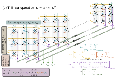
## Diagram: Trilinear Operation (O = A · B · C^T) ### Overview The diagram illustrates a trilinear operation involving three matrices (A, B, C) and their interaction to produce an output O. It depicts a three-stage processing pipeline with labeled components, mathematical relationships, and data flow. The operation is defined as a tensor contraction across three dimensions, with explicit voltage-controlled inputs and output summation. ### Components/Axes 1. **Title**: "Trilinear operation: O = A · B · C^T" (top-left) 2. **Stages**: - **Stage 1 (Left)**: - **Backgate input**: Labeled as "(a₁₁…a₁₂) via V_AC" (green arrows) - **Sequence input**: Labeled as "(a₁₁…a₁₂) via V_AC" (blue arrows) - **Weighted Non-volatility C**: Labeled as "via V_TG" (orange arrows) - **Stage 2 (Center)**: - **Addition nodes**: Labeled "Addition" (gray dashed lines) - **Stage 3 (Right)**: - **Output nodes**: Labeled "Trilinear output" (purple arrows) 3. **Mathematical Expressions**: - Trilinear output formula: $ o_{r^{\prime}i^{\prime}} = \sum_{j=1}^{N_2} \sum_{k=1}^{D_3} a_{r^{\prime}j} b_{j k} c_{i' k} $ - Matrix definitions: - $ A = \begin{bmatrix} a_{11} & \cdots & a_{1N_2} \\ \vdots & \ddots & \vdots \\ a_{N_11} & \cdots & a_{N_1N_2} \end{bmatrix} $ - $ B = \begin{bmatrix} b_{11} & \cdots & b_{1D_2} \\ \vdots & \ddots & \vdots \\ b_{D_1} & \cdots & b_{D_1D_2} \end{bmatrix} $ - $ C^T = \begin{bmatrix} c_{11} & \cdots & c_{1D_3} \\ \vdots & \ddots & \vdots \\ c_{D_2} & \cdots & c_{D_2D_3} \end{bmatrix} $ - Output matrix: $ O = \begin{bmatrix} o_{11} & \cdots & o_{1D_3} \\ \vdots & \ddots & \vdots \\ o_{N_1} & \cdots & o_{N_1D_3} \end{bmatrix} $ ### Detailed Analysis - **Data Flow**: - Backgate and sequence inputs (Stage 1) feed into weighted non-volatility C (Stage 1), which propagates through addition nodes (Stage 2) to produce the trilinear output (Stage 3). - Voltage-controlled inputs (V_AC, V_TG) modulate the interaction between matrices. - **Matrix Dimensions**: - $ A \in \mathbb{R}^{N_1 \times N_2} $, $ B \in \mathbb{R}^{D_1 \times D_2} $, $ C^T \in \mathbb{R}^{D_2 \times D_3} $, with $ N_1 = N_2 = D_1 = D_2 = D_3 $ (explicitly stated in the diagram). - **Output Structure**: - The trilinear output $ O $ is a $ N_1 \times D_3 $ matrix, computed via nested summations over $ j $ and $ k $. ### Key Observations - **Symmetry**: The diagram emphasizes symmetry in matrix dimensions ($ N_1 = N_2 = D_1 = D_2 = D_3 $), simplifying the trilinear contraction. - **Non-Volatility**: The term "Weighted Non-volatility C" suggests a hardware-aware design, possibly for energy-efficient computation. - **Addition Nodes**: The central stage aggregates intermediate results, indicating a parallel processing architecture. ### Interpretation This diagram represents a **tensor-based computational model** for trilinear operations, likely in the context of neuromorphic or analog computing. The use of voltage-controlled inputs (V_AC, V_TG) implies a physical implementation where electrical signals modulate matrix interactions. The operation combines three matrices (A, B, C) through element-wise multiplication and summation, producing a compact output matrix $ O $. The explicit dimension constraints ($ N_1 = N_2 = D_1 = D_2 = D_3 $) suggest a balanced design for efficient computation, avoiding redundant dimensions. The "Weighted Non-volatility C" component hints at a focus on energy efficiency, as non-volatile memory elements retain state without power, reducing dynamic energy consumption. This model could be applied to tasks like signal processing, machine learning, or quantum computing, where trilinear operations are fundamental.