## Line Chart: Two-Timescale Dissociation: Transient Compression vs Persistent Spectral Shape
### Overview
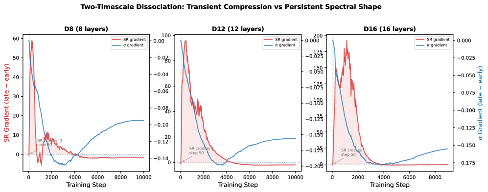
The image contains three line charts (D8, D12, D16) comparing the evolution of two gradients ("SR gradient" and "α gradient") during training steps. Each subplot represents a different model architecture with varying layer counts (8, 12, 16 layers). The charts visualize how these gradients change over training iterations, with annotations highlighting key events (e.g., "SR crosses 0 step 50").
---
### Components/Axes
1. **X-Axis**:
- Label: "Training Step"
- Scale: 0 to 10,000 (linear)
2. **Y-Axes**:
- **Left Y-Axis (SR Gradient)**:
- Label: "SR Gradient (late – early)"
- Scale:
- D8: 0–60
- D12: 0–100
- D16: 0–200
- **Right Y-Axis (α Gradient)**:
- Label: "α Gradient (late – early)"
- Scale: -0.25 to 0 (consistent across all subplots)
3. **Legends**:
- Position: Top-right of each subplot
- Colors:
- Red: "SR gradient"
- Blue: "α gradient"
4. **Annotations**:
- "SR crosses 0 step 50" (arrow pointing to SR gradient crossing zero at step 50)
---
### Detailed Analysis
#### D8 (8 layers)
- **SR Gradient (Red)**:
- Starts at ~60, drops sharply to ~0 by step 50, then stabilizes near 0.
- Shaded region (confidence interval) narrows significantly after step 50.
- **α Gradient (Blue)**:
- Starts at ~-0.25, rises to ~-0.1 by step 50, then plateaus.
- Shaded region widens initially, then narrows.
#### D12 (12 layers)
- **SR Gradient (Red)**:
- Starts at ~100, drops to ~0 by step 50, then stabilizes.
- Shaded region shows high variability early, then stabilizes.
- **α Gradient (Blue)**:
- Starts at ~-0.25, rises to ~-0.12 by step 50, then plateaus.
- Shaded region narrows gradually.
#### D16 (16 layers)
- **SR Gradient (Red)**:
- Starts at ~175, drops to ~0 by step 50, then stabilizes.
- Shaded region shows extreme early variability, then stabilizes.
- **α Gradient (Blue)**:
- Starts at ~-0.25, rises to ~-0.15 by step 50, then plateaus.
- Shaded region narrows sharply after step 50.
---
### Key Observations
1. **SR Gradient Behavior**:
- All subplots show a sharp decline in SR gradient to near zero by step 50, followed by stabilization.
- Larger models (D16) exhibit higher initial SR gradient values and more pronounced variability.
2. **α Gradient Behavior**:
- α gradient consistently starts at ~-0.25 and rises gradually across all subplots.
- Larger models (D16) show a steeper rise in α gradient post-step 50.
3. **Crossing Point**:
- SR gradient crosses zero at step 50 in all subplots, coinciding with a critical transition in training dynamics.
4. **Shaded Regions**:
- Reflect uncertainty/variability, which decreases as training progresses.
---
### Interpretation
1. **Transient Compression (SR Gradient)**:
- The sharp decline in SR gradient suggests early-stage transient compression of spectral features, which stabilizes as training progresses. Larger models (D16) require more training steps to achieve stability.
2. **Persistent Spectral Shape (α Gradient)**:
- The gradual rise in α gradient indicates persistent spectral shape adjustments, which become more pronounced in larger models. This suggests that deeper architectures require more extensive spectral adaptation.
3. **Model Complexity and Training Dynamics**:
- Larger models (D16) exhibit higher initial gradient magnitudes and greater variability, implying that increased complexity introduces more instability during early training.
- The crossing of SR gradient at step 50 marks a phase transition where transient effects diminish, and persistent spectral adjustments dominate.
4. **Practical Implications**:
- The data highlights the importance of monitoring both transient (SR) and persistent (α) spectral dynamics during training.
- Larger models may require adjusted training schedules or regularization to manage early instability.
---
**Note**: All values are approximate, derived from visual inspection of the chart. Uncertainty is represented by shaded regions and variability in gradient trajectories.