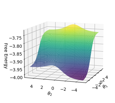
\n ## 3D Surface Plot: Free Energy Landscape ### Overview The image displays a three-dimensional surface plot visualizing "Free Energy" as a function of two parameters, θ₁ and θ₂. The plot is rendered in a perspective view, showing a continuous, curved surface that represents the relationship between the three variables. The surface is colored with a gradient that maps to the Free Energy value. ### Components/Axes * **Vertical Axis (Z-axis):** * **Label:** "Free Energy" * **Scale:** Linear, ranging from approximately **-4.00** at the bottom to **-3.75** at the top. * **Markers:** Major ticks are visible at -4.00, -3.95, -3.90, -3.85, -3.80, and -3.75. * **Horizontal Axis 1 (X-axis, front-right):** * **Label:** "θ₁" (Theta subscript 1) * **Scale:** Linear, ranging from **-4** to **4**. * **Markers:** Major ticks at -4, -2, 0, 2, 4. * **Horizontal Axis 2 (Y-axis, front-left):** * **Label:** "θ₂" (Theta subscript 2) * **Scale:** Linear, ranging from **-4** to **4**. * **Markers:** Major ticks at -4, -2, 0, 2, 4. * **Color Mapping (Implicit Legend):** * The surface color corresponds directly to the Free Energy (Z) value. * **Dark Purple/Blue:** Represents the lowest Free Energy values (near **-4.00**). * **Teal/Green:** Represents mid-range Free Energy values (around **-3.90**). * **Yellow:** Represents the highest Free Energy values (near **-3.75**). ### Detailed Analysis The surface forms a smooth, continuous landscape with a distinct topological feature. * **Global Minimum:** The lowest point on the surface (deepest purple) is located at the coordinate **(θ₁ ≈ 0, θ₂ ≈ 0)**. The Free Energy at this point is approximately **-4.00**. * **General Trend:** Moving away from the origin (0,0) in any direction along the θ₁-θ₂ plane generally results in an increase in Free Energy. The surface slopes upward from the central minimum. * **Asymmetry and Ridge:** The increase is not uniform. There is a pronounced ridge or saddle point running diagonally. The surface rises more steeply towards the positive θ₁, positive θ₂ quadrant (back corner) and the negative θ₁, negative θ₂ quadrant (front corner), reaching its highest values (yellow) in these regions. The rise is more gradual along the anti-diagonal (positive θ₁, negative θ₂ and negative θ₁, positive θ₂). * **Spatial Grounding:** The highest point (yellow) appears to be near **(θ₁ ≈ 4, θ₂ ≈ 4)** and **(θ₁ ≈ -4, θ₂ ≈ -4)**, with Free Energy values approaching **-3.75**. The lowest point is clearly at the center of the grid. ### Key Observations 1. **Single Well Potential:** The landscape depicts a single, broad energy well centered at the origin, suggesting a stable equilibrium point at (0,0). 2. **Anisotropic Curvature:** The "walls" of the well are not symmetrical. The curvature is tighter (steeper slope) along the θ₁ = θ₂ diagonal compared to the θ₁ = -θ₂ diagonal. 3. **No Local Minima:** Within the plotted range, there are no other local minima or maxima besides the global minimum at the center. The surface is smooth and convex in the region shown. ### Interpretation This plot likely represents an **energy landscape or cost function** from fields like statistical mechanics, optimization theory, or machine learning. * **What it demonstrates:** The function has a clear, unique minimum at θ₁ = 0, θ₂ = 0. This is the optimal state where the system's "Free Energy" (or cost, error) is minimized. Any deviation from these parameter values increases the energy/cost. * **Relationship between elements:** The two parameters θ₁ and θ₂ are coupled. Changing one affects the Free Energy, and the effect depends on the value of the other parameter, as shown by the curved, non-planar surface. The diagonal ridge indicates that certain combinations of parameters (e.g., both large and positive) are particularly "costly." * **Potential Context:** In an optimization context, this would be a straightforward landscape to minimize using gradient-based methods, as there are no deceptive local minima. In a physical context, it could represent the free energy of a system as a function of two order parameters, with (0,0) being the stable phase. The asymmetry suggests the system's response to perturbations is direction-dependent.