## Mathematical Commutative Diagram: Relationship Between Curve Spaces and Loss Functions
### Overview
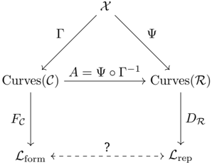
The image displays a commutative diagram from mathematics, likely from category theory, algebraic geometry, or machine learning theory. It illustrates the relationships between several abstract objects (represented as nodes) and the mappings (morphisms) between them. The diagram has a triangular upper section and a rectangular lower section, connected by vertical arrows. A dashed arrow with a question mark indicates an unknown or conjectured relationship.
### Components/Axes
The diagram consists of five nodes and six labeled arrows (morphisms).
**Nodes (Objects):**
1. **X**: Positioned at the top center.
2. **Curves(C)**: Positioned at the middle left.
3. **Curves(R)**: Positioned at the middle right.
4. **L_form**: Positioned at the bottom left.
5. **L_rep**: Positioned at the bottom right.
**Arrows (Morphisms) and Labels:**
1. **Γ (Gamma)**: A solid arrow pointing from **X** down-left to **Curves(C)**.
2. **Ψ (Psi)**: A solid arrow pointing from **X** down-right to **Curves(R)**.
3. **A = Ψ ∘ Γ⁻¹**: A solid horizontal arrow pointing from **Curves(C)** to **Curves(R)**. The label defines `A` as the composition of `Ψ` and the inverse of `Γ`.
4. **F_C**: A solid vertical arrow pointing down from **Curves(C)** to **L_form**.
5. **D_R**: A solid vertical arrow pointing down from **Curves(R)** to **L_rep**.
6. **?**: A dashed horizontal arrow pointing from **L_form** to **L_rep**. The question mark indicates this relationship is unknown, to be determined, or is the subject of inquiry.
### Detailed Analysis
The diagram defines a structured relationship between abstract spaces:
* The object **X** maps via two different functions, **Γ** and **Ψ**, into two spaces of "curves," **Curves(C)** and **Curves(R)**. The letters `C` and `R` likely denote different underlying fields (e.g., Complex and Real numbers) or categories.
* A direct mapping **A** between the two curve spaces is explicitly defined as the composition `Ψ ∘ Γ⁻¹`. This implies that **Γ** is assumed to be invertible (an isomorphism) for this definition to hold.
* From each curve space, a further mapping leads to a "loss" or "objective" space: **F_C** maps from **Curves(C)** to **L_form**, and **D_R** maps from **Curves(R)** to **L_rep**. The subscripts `form` and `rep` might stand for "formulation" and "representation," or similar conceptual distinctions.
* The core of the diagram's inquiry is represented by the dashed arrow **?**. It asks whether there is a well-defined, natural, or commutative relationship between the two loss spaces **L_form** and **L_rep**. The diagram's commutativity (or lack thereof) for the lower square is the central question.
### Key Observations
1. **Hierarchical Structure**: The diagram has a clear top-down flow from the abstract object **X** to the concrete loss spaces **L_form** and **L_rep**.
2. **Symmetry and Asymmetry**: The upper triangle (X, Curves(C), Curves(R)) is symmetric in its construction from **X**. The lower rectangle is asymmetric due to the different labels on the vertical arrows (**F_C** vs. **D_R**) and the unknown horizontal link.
3. **Critical Dependency**: The definition of the horizontal map **A** depends entirely on the invertibility of **Γ**. If **Γ** is not invertible, this map is not well-defined as stated.
4. **Central Unknown**: The dashed arrow with the question mark is the focal point. It highlights a gap in knowledge or a proposition to be proven: whether the two paths from the curve spaces to the loss spaces are connected in a meaningful way.
### Interpretation
This diagram formalizes a problem of **translating or comparing two different formulations of a problem**. One starts with a common source **X** (e.g., a dataset, a geometric object, a theoretical construct) and processes it through two different lenses or frameworks, represented by **Γ** and **Ψ**, resulting in two different "curve" representations.
The subsequent steps, **F_C** and **D_R**, likely represent the computation of a loss, error, or objective function specific to each framework. The ultimate question posed by the diagram is: **Are the resulting loss landscapes (L_form and L_rep) related?** Can one be transformed into the other? Is there a guarantee that optimizing one corresponds to optimizing the other?
The diagram suggests that if the initial mappings are well-behaved (i.e., **Γ** is invertible, allowing the definition of **A**), then one might hope for a relationship between the final outputs. The dashed line **?** represents the hypothesis, theorem, or research question that seeks to establish this connection, which would be crucial for ensuring consistency between different methodological approaches.