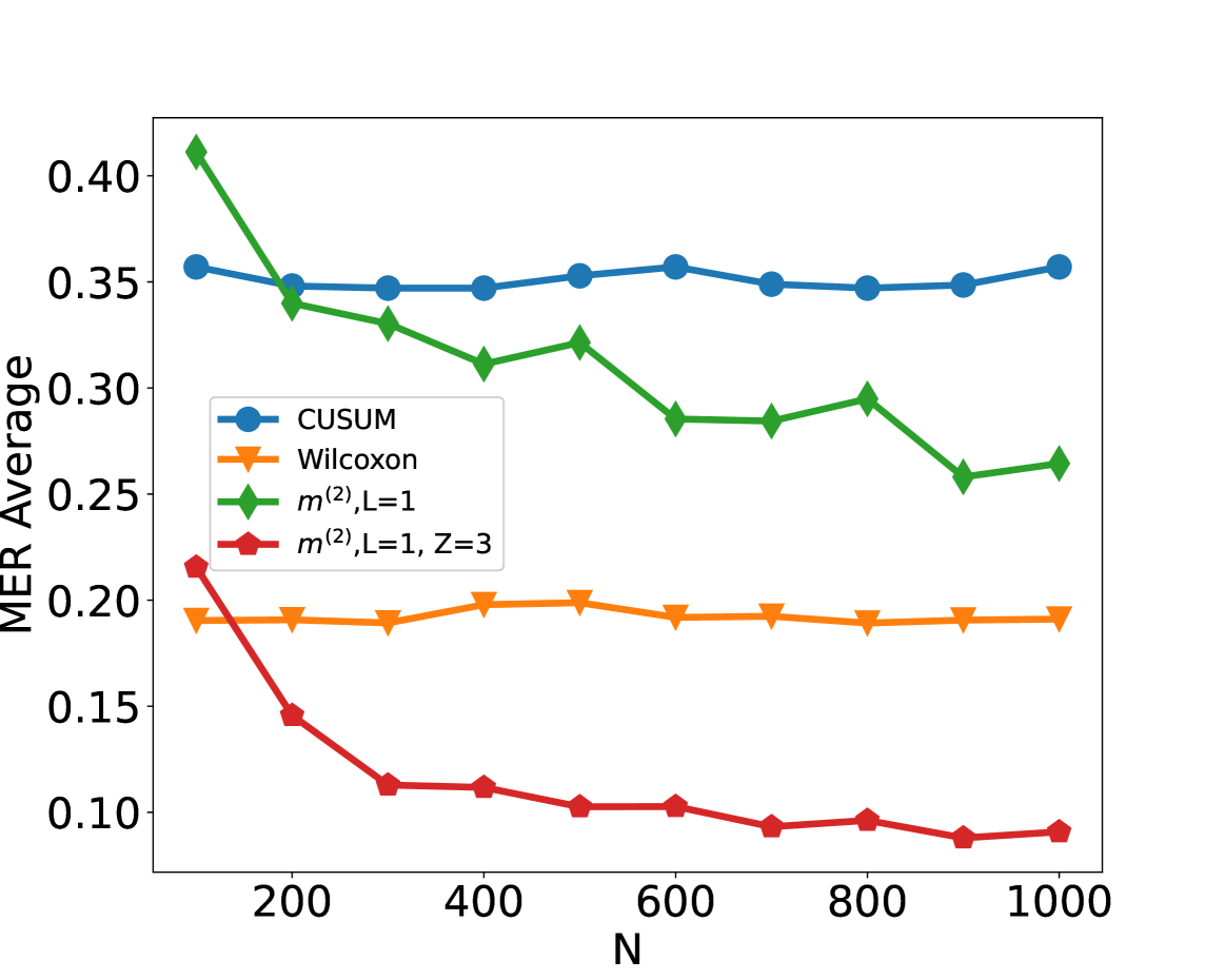
## Line Chart: MER Average vs. N
### Overview
The image displays a line chart comparing the performance of four different statistical methods or algorithms. The performance metric is "MER Average" plotted against a variable "N," which likely represents sample size, number of observations, or a similar parameter. The chart shows how the average MER (a metric whose exact definition is not provided) changes for each method as N increases from approximately 100 to 1000.
### Components/Axes
* **X-Axis:** Labeled **"N"**. The axis has major tick marks at 200, 400, 600, 800, and 1000. The data points appear to be plotted at intervals of 100, starting from N=100.
* **Y-Axis:** Labeled **"MER Average"**. The axis has major tick marks at 0.10, 0.15, 0.20, 0.25, 0.30, 0.35, and 0.40.
* **Legend:** Located in the **top-left quadrant** of the chart area. It contains four entries, each associating a color, marker shape, and label:
1. **Blue line with circle markers:** `CUSUM`
2. **Orange line with downward-pointing triangle markers:** `Wilcoxon`
3. **Green line with diamond markers:** `m^(2), L=1`
4. **Red line with pentagon markers:** `m^(2), L=1, Z=3`
### Detailed Analysis
**Data Series Trends and Approximate Values:**
1. **CUSUM (Blue, Circles):**
* **Trend:** The line is remarkably flat and stable across all values of N.
* **Data Points (Approximate):** Starts at ~0.36 (N=100), remains between ~0.35 and ~0.36 for all subsequent points (N=200 to N=1000).
2. **Wilcoxon (Orange, Triangles):**
* **Trend:** Also very stable, forming a nearly horizontal line, but at a significantly lower MER Average than CUSUM.
* **Data Points (Approximate):** Hovers consistently around ~0.19 to ~0.20 from N=100 to N=1000.
3. **m^(2), L=1 (Green, Diamonds):**
* **Trend:** Shows a clear downward trend. It starts as the highest value and decreases as N increases, with some minor fluctuations (e.g., a slight rise at N=500 and N=800).
* **Data Points (Approximate):** Starts at ~0.41 (N=100), drops to ~0.34 (N=200), ~0.33 (N=300), ~0.31 (N=400), ~0.32 (N=500), ~0.29 (N=600), ~0.29 (N=700), ~0.30 (N=800), ~0.26 (N=900), and ends at ~0.27 (N=1000).
4. **m^(2), L=1, Z=3 (Red, Pentagons):**
* **Trend:** Exhibits the most pronounced downward trend, especially for smaller N. It starts at a moderate level and decreases rapidly before leveling off at a very low MER Average.
* **Data Points (Approximate):** Starts at ~0.22 (N=100), drops sharply to ~0.15 (N=200), ~0.11 (N=300), ~0.11 (N=400), ~0.10 (N=500), ~0.10 (N=600), ~0.09 (N=700), ~0.10 (N=800), ~0.09 (N=900), and ends at ~0.09 (N=1000).
### Key Observations
* **Performance Hierarchy:** For all N > 100, the methods rank from highest to lowest MER Average as: CUSUM > m^(2), L=1 > Wilcoxon > m^(2), L=1, Z=3.
* **Stability vs. Improvement:** CUSUM and Wilcoxon show stable performance independent of N. In contrast, both `m^(2)` variants show improvement (decreasing MER Average) as N increases.
* **Impact of Z Parameter:** The addition of the `Z=3` parameter to the `m^(2), L=1` method (red line) dramatically improves its performance, lowering its MER Average significantly compared to the base version (green line) across all N.
* **Convergence:** The red line (`m^(2), L=1, Z=3`) appears to converge to a floor value of approximately 0.09 for N ≥ 700.
### Interpretation
This chart likely evaluates the efficiency or error rate (where lower MER is better) of different change-point detection or statistical testing algorithms as the amount of data (N) grows.
* The **CUSUM** method is robust and consistent but has a relatively high average MER, suggesting it may be less sensitive or have a higher baseline error in this specific context.
* The **Wilcoxon** method is also stable but performs better than CUSUM, indicating it might be a more suitable non-parametric test for this scenario.
* The **`m^(2)`** methods demonstrate a desirable property: their performance improves with more data. The base `m^(2), L=1` starts poorly but becomes competitive with Wilcoxon for large N.
* The most significant finding is the **superior performance of `m^(2), L=1, Z=3`**. The `Z=3` parameter (which could represent a threshold, window size, or tuning parameter) is crucial, transforming the method into the best-performing one for all N > 100. It achieves the lowest MER Average and shows the fastest rate of improvement, making it the most effective algorithm among those compared for this task, especially when sufficient data is available. The chart makes a strong case for using this specific parameterization of the `m^(2)` method.