# Technical Document Extraction: 2D Spatial Estimation Plot
## 1. Component Isolation
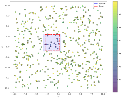
The image is a 2D scatter plot representing a spatial distribution of data points with overlaid estimation regions and a color-coded intensity scale.
* **Header/Legend Region:** Located at the top right of the main axes.
* **Main Chart Region:** A square coordinate system ranging from -10 to 10 on both axes.
* **Colorbar/Scale Region:** A vertical bar located to the right of the main chart.
---
## 2. Metadata and Labels
* **X-axis Label ($x_0$):** Horizontal axis, ranging from -10.0 to 10.0.
* **Y-axis Label ($x_1$):** Vertical axis, ranging from -10.0 to 10.0.
* **Legend (Top Right):**
* **Blue Solid Line:** $S$ (True) - Represents the ground truth boundary.
* **Red Solid Line:** $\hat{S}$ (Est) - Represents the estimated boundary.
* **Colorbar (Right):** A continuous vertical scale ranging from approximately **0.3** (dark purple) to **1.0** (bright yellow).
---
## 3. Data Series and Visual Trends
### A. Scatter Points (Data Distribution)
* **Trend:** The points are distributed quasi-randomly across the entire $20 \times 20$ unit field.
* **Color Mapping:**
* Points outside the central region are primarily colored in the **green-to-yellow** spectrum (values $\approx 0.7$ to $1.0$ on the colorbar).
* Points located within the central bounded region are colored in the **dark purple-to-blue** spectrum (values $\approx 0.3$ to $0.5$ on the colorbar).
* **Observation:** There is a clear correlation between spatial location and the value represented by the color; the central "box" contains significantly lower values than the surrounding field.
### B. Boundary Regions (The "Boxes")
There are two overlapping rectangular regions centered near the origin:
1. **True Boundary ($S$):**
* **Visual:** A light blue/lavender shaded rectangle with a faint blue dashed border.
* **Spatial Grounding:** Extends approximately from **-3.5 to 0.5** on the $x_0$ axis and **-1.0 to 3.0** on the $x_1$ axis.
2. **Estimated Boundary ($\hat{S}$):**
* **Visual:** A thick, red dashed line forming a rectangle.
* **Spatial Grounding:** Extends approximately from **-3.0 to 0.3** on the $x_0$ axis and **-0.8 to 3.0** on the $x_1$ axis.
* **Trend:** The estimated boundary ($\hat{S}$) is slightly smaller than the true boundary ($S$) but captures the majority of the low-value (purple) data points.
---
## 4. Detailed Data Extraction
### Axis Markers
| Axis | Min Value | Max Value | Major Increments |
| :--- | :--- | :--- | :--- |
| **$x_0$ (Horizontal)** | -10.0 | 10.0 | 2.5 |
| **$x_1$ (Vertical)** | -10.0 | 10.0 | 2.5 |
### Region Coordinates (Approximate)
| Feature | $x_0$ Range | $x_1$ Range | Visual Style |
| :--- | :--- | :--- | :--- |
| **True Region ($S$)** | [-3.5, 0.5] | [-1.0, 3.0] | Light Blue Fill, Blue Dash |
| **Estimated Region ($\hat{S}$)** | [-3.0, 0.3] | [-0.8, 3.0] | Red Dash |
---
## 5. Summary of Information
This chart visualizes a classification or estimation task. The goal appears to be identifying a specific spatial region (the "True" box) where data values (represented by color) are significantly lower than the background.
* **Background Values:** High (Yellow/Green, $\approx 0.85$).
* **Target Region Values:** Low (Purple/Blue, $\approx 0.4$).
* **Estimation Performance:** The red dashed box ($\hat{S}$) provides a high-accuracy estimation of the true region ($S$), with a slight under-estimation on the left and bottom edges.