## Line Chart: Accuracy vs. Time
### Overview
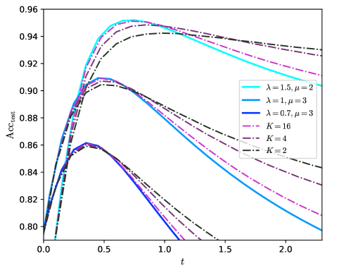
The image presents a line chart illustrating the relationship between accuracy (Acc_test) and time (t) for different parameter settings. Several lines represent different combinations of λ, μ, and K values. The chart appears to model a learning or convergence process, where accuracy increases initially and then plateaus or declines.
### Components/Axes
* **X-axis:** Labeled as "t", ranging from approximately 0.0 to 2.2.
* **Y-axis:** Labeled as "Acc_test", ranging from approximately 0.80 to 0.96.
* **Legend:** Located in the top-right corner, containing the following lines and their corresponding parameters:
* λ = 1.5, μ = 2 (Light Blue, Solid)
* λ = 1, μ = 3 (Blue, Solid)
* λ = 0.7, μ = 3 (Dark Blue, Solid)
* K = 16 (Pink, Dashed)
* K = 4 (Purple, Dashed)
* K = 2 (Black, Dashed)
### Detailed Analysis
Let's analyze each line's trend and approximate data points:
* **λ = 1.5, μ = 2 (Light Blue, Solid):** This line starts at approximately Acc_test = 0.81 at t = 0.0. It increases rapidly, reaching a peak of approximately Acc_test = 0.95 at t ≈ 0.6. After the peak, it gradually declines to approximately Acc_test = 0.94 at t = 2.0.
* **λ = 1, μ = 3 (Blue, Solid):** This line begins at approximately Acc_test = 0.81 at t = 0.0. It rises quickly, peaking at approximately Acc_test = 0.95 at t ≈ 0.5. It then decreases slowly, reaching approximately Acc_test = 0.94 at t = 2.0.
* **λ = 0.7, μ = 3 (Dark Blue, Solid):** Starting at approximately Acc_test = 0.81 at t = 0.0, this line increases to a peak of approximately Acc_test = 0.92 at t ≈ 0.4. It then declines more rapidly than the other two lines, reaching approximately Acc_test = 0.90 at t = 2.0.
* **K = 16 (Pink, Dashed):** This line starts at approximately Acc_test = 0.86 at t = 0.0. It increases to a peak of approximately Acc_test = 0.94 at t ≈ 0.7. It then declines slowly, reaching approximately Acc_test = 0.93 at t = 2.0.
* **K = 4 (Purple, Dashed):** Beginning at approximately Acc_test = 0.85 at t = 0.0, this line rises to a peak of approximately Acc_test = 0.92 at t ≈ 0.6. It then declines more noticeably, reaching approximately Acc_test = 0.90 at t = 2.0.
* **K = 2 (Black, Dashed):** This line starts at approximately Acc_test = 0.84 at t = 0.0. It increases to a peak of approximately Acc_test = 0.89 at t ≈ 0.5. It then declines, reaching approximately Acc_test = 0.86 at t = 2.0.
### Key Observations
* The lines representing different values of λ and μ generally exhibit a similar trend: initial increase followed by a plateau or decline.
* Higher values of λ and μ (e.g., λ = 1.5, μ = 2 and λ = 1, μ = 3) tend to achieve higher peak accuracies.
* The lines representing different values of K show a similar trend, but generally achieve lower peak accuracies compared to the λ and μ lines.
* The line for K = 2 consistently shows the lowest accuracy throughout the entire time range.
* The lines for K = 16 and K = 4 have similar trajectories, peaking around the same accuracy level.
### Interpretation
The chart likely represents the performance of a model or algorithm over time, where λ, μ, and K are hyperparameters controlling its behavior. The Acc_test metric indicates the accuracy of the model on a test dataset.
The data suggests that:
* Increasing λ and μ generally improves the model's accuracy, at least initially.
* The value of K has a significant impact on accuracy, with higher values of K leading to better performance (up to a certain point).
* The decline in accuracy after the peak could indicate overfitting, where the model starts to perform worse on unseen data as it becomes too specialized to the training data.
* The different lines represent different configurations of the model, and the chart allows for a comparison of their performance under different conditions.
The chart provides valuable insights into the sensitivity of the model's performance to different hyperparameters, which can be used to optimize its configuration for better accuracy and generalization ability. The fact that all lines eventually decline suggests a need for regularization or other techniques to prevent overfitting.