## Chart: gSSNR gain vs TotERITF ### Overview The image is a line chart comparing the performance of different algorithms (JBLCMV, Prop, BMVDR, BLCMV, OBLCMV) in terms of gSSNR gain (dB) versus TotERITF. The chart displays multiple data series, each representing a different algorithm or configuration. The x-axis represents TotERITF, and the y-axis represents gSSNR gain in dB. ### Components/Axes * **X-axis:** TotERITF, ranging from 0 to approximately 90. * **Y-axis:** gSSNR gain (dB), ranging from 0 to 35. * **Title:** gSSNR gain (dB) vs TotERITF (inferred from axis labels and context). * **Legend (Top-Right):** * Red triangle: JBLCMV * Blue triangle: Prop.-c = 0.3, kmax = 10 * Magenta x: Prop.-c = 0.3, kmax = 50 * Light green star: Prop.-c = 0.6, kmax = 10 * Yellow circle: Prop.-c = 0.6, kmax = 50 * Black diamond: BMVDR * Brown square: BLCMV-η = 0.1 * Red plus: BLCMV-η = 0.001 * Dark green asterisk: OBLCMV ### Detailed Analysis * **JBLCMV (Red Triangles):** Starts at approximately (0, 4) and increases slightly before decreasing and remaining relatively flat around 2-4 dB. * **Prop.-c = 0.3, kmax = 10 (Blue Triangles):** Starts at approximately (0, 5) and increases to approximately (15, 6) before decreasing and remaining relatively flat around 4-6 dB. * **Prop.-c = 0.3, kmax = 50 (Magenta x):** Starts at approximately (0, 6) and increases to approximately (15, 5) before decreasing and remaining relatively flat around 2-5 dB. * **Prop.-c = 0.6, kmax = 10 (Light green star):** Starts at approximately (0, 7) and increases to approximately (40, 6) before decreasing and remaining relatively flat around 4-7 dB. * **Prop.-c = 0.6, kmax = 50 (Yellow circle):** Starts at approximately (0, 7) and increases to approximately (40, 5) before decreasing and remaining relatively flat around 4-6 dB. * **BMVDR (Black Diamonds):** Starts at approximately (0, 20) and decreases sharply to approximately (5, 8) before increasing and remaining relatively flat around 6-8 dB. * **BLCMV-η = 0.1 (Brown Squares):** Starts at approximately (0, 15) and decreases sharply to approximately (5, 7) before increasing and remaining relatively flat around 6-7 dB. * **BLCMV-η = 0.001 (Red Plus):** Starts at approximately (0, 30) and decreases sharply to approximately (5, 7) before increasing and remaining relatively flat around 6-7 dB. * **OBLCMV (Dark green Asterisk):** Starts at approximately (0, 33) and decreases sharply to approximately (5, 8) before increasing and remaining relatively flat around 6-8 dB. ### Key Observations * The algorithms OBLCMV, BLCMV-η = 0.001, and BMVDR show the highest initial gSSNR gain but experience a sharp decrease as TotERITF increases. * The "Prop" algorithms generally have lower initial gSSNR gain but maintain a more stable performance as TotERITF increases. * All algorithms tend to converge to a relatively flat gSSNR gain as TotERITF increases beyond 20. ### Interpretation The chart illustrates a trade-off between initial gSSNR gain and stability with respect to TotERITF. Algorithms like OBLCMV and BMVDR offer high initial gain but are more sensitive to changes in TotERITF. In contrast, the "Prop" algorithms provide a more consistent performance across different TotERITF values, albeit at a lower initial gain. The choice of algorithm would depend on the specific application and the importance of initial gain versus stability. The BLCMV algorithms perform similarly to BMVDR and OBLCMV.

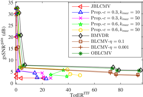
\n ## Chart: gSSNR Gain vs. TotERITF ### Overview The image presents a line chart illustrating the relationship between gSSNR gain (in dB) and TotERITF. The chart compares the performance of several different algorithms or configurations, indicated by different colored lines and markers. The x-axis represents TotERITF, and the y-axis represents gSSNR gain. ### Components/Axes * **X-axis:** TotERITF (ranging from 0 to approximately 90). * **Y-axis:** gSSNR gain (dB) (ranging from 0 to approximately 35). * **Legend (top-right):** Contains labels for each data series, with corresponding colors and markers: * JBLCMV (Red, Triangle) * Prop.-c = 0.3, kmax = 10 (Magenta, X) * Prop.-c = 0.3, kmax = 50 (Cyan, Star) * Prop.-c = 0.6, kmax = 10 (Yellow, Circle) * Prop.-c = 0.6, kmax = 50 (Black, Diamond) * BMVDR (Brown, Square) * BLCMV-η = 0.1 (Orange, Square) * BLCMV-η = 0.001 (Dark Red, Square) * OBLCMV (Green, Asterisk) ### Detailed Analysis The chart displays several lines, each representing a different algorithm's performance. * **OBLCMV (Green Asterisk):** Starts at approximately 31 dB at TotERITF = 0, rapidly decreasing to approximately 5 dB at TotERITF = 10, and then leveling off around 4-5 dB for the remainder of the range. * **BMVDR (Brown Square):** Starts at approximately 21 dB at TotERITF = 0, decreases sharply to approximately 7 dB at TotERITF = 10, and then remains relatively stable around 6-8 dB. * **JBLCMV (Red Triangle):** Starts at approximately 3 dB at TotERITF = 0, increases slightly to around 4 dB at TotERITF = 10, and then remains relatively stable around 3-4 dB. * **Prop.-c = 0.3, kmax = 10 (Magenta X):** Starts at approximately 5 dB at TotERITF = 0, decreases to around 3 dB at TotERITF = 10, and then remains relatively stable around 3-4 dB. * **Prop.-c = 0.3, kmax = 50 (Cyan Star):** Starts at approximately 5 dB at TotERITF = 0, decreases to around 3 dB at TotERITF = 10, and then remains relatively stable around 3-4 dB. * **Prop.-c = 0.6, kmax = 10 (Yellow Circle):** Starts at approximately 4 dB at TotERITF = 0, decreases to around 3 dB at TotERITF = 10, and then remains relatively stable around 3-4 dB. * **Prop.-c = 0.6, kmax = 50 (Black Diamond):** Starts at approximately 4 dB at TotERITF = 0, decreases to around 3 dB at TotERITF = 10, and then remains relatively stable around 3-4 dB. * **BLCMV-η = 0.1 (Orange Square):** Starts at approximately 6 dB at TotERITF = 0, decreases to around 4 dB at TotERITF = 10, and then remains relatively stable around 4-5 dB. * **BLCMV-η = 0.001 (Dark Red Square):** Starts at approximately 6 dB at TotERITF = 0, decreases to around 4 dB at TotERITF = 10, and then remains relatively stable around 3-4 dB. ### Key Observations * OBLCMV exhibits the highest initial gSSNR gain but experiences the most significant drop as TotERITF increases. * JBLCMV, Prop.-c = 0.3, kmax = 10, Prop.-c = 0.3, kmax = 50, Prop.-c = 0.6, kmax = 10, Prop.-c = 0.6, kmax = 50, BLCMV-η = 0.001 show very similar performance, remaining relatively stable at low gSSNR gain values (around 3-4 dB) after an initial decrease. * BMVDR and BLCMV-η = 0.1 show intermediate performance, with a more moderate decrease in gSSNR gain as TotERITF increases. ### Interpretation The chart demonstrates the performance trade-offs between different algorithms for signal processing, likely in a noisy environment. The gSSNR gain represents the improvement in signal-to-noise ratio achieved by each algorithm. TotERITF likely represents a measure of environmental or interference characteristics. The rapid decline in gSSNR gain for OBLCMV suggests that it is highly sensitive to increasing TotERITF, meaning its performance degrades significantly as the interference level rises. Conversely, the algorithms with stable performance (JBLCMV, Prop.-c variants, BLCMV-η = 0.001) are more robust to changes in TotERITF, maintaining a consistent level of noise reduction. The differences between the Prop.-c and kmax parameter settings suggest that these parameters influence the algorithm's sensitivity to interference. The relatively similar performance of the Prop.-c variants indicates that the specific parameter values chosen have a limited impact on overall performance within the tested range. The chart suggests that the choice of algorithm should be based on the expected level of interference (TotERITF). If the interference level is expected to be high, a more robust algorithm (e.g., JBLCMV) would be preferable, even if it offers lower initial gSSNR gain. If the interference level is low, OBLCMV might be a good choice due to its higher initial performance.

## Line Graph: gSSNR Gain vs. TotER_ITF ### Overview The graph compares the gSSNR gain (in dB) across multiple configurations as a function of TotER_ITF. It features seven distinct data series with varying trends, plotted using different symbols and colors. The y-axis ranges from 0 to 35 dB, while the x-axis spans 0 to 80 TotER_ITF. ### Components/Axes - **X-axis**: Labeled "TotER_ITF" with ticks at 0, 20, 40, 60, and 80. - **Y-axis**: Labeled "gSSNR_gain (dB)" with ticks at 0, 5, 10, 15, 20, 25, and 35. - **Legend**: Positioned in the top-right corner, containing seven entries: 1. **JBLCMV** (red triangle) 2. **Prop.-c = 0.3, k_max = 10** (blue triangle) 3. **Prop.-c = 0.3, k_max = 50** (pink cross) 4. **Prop.-c = 0.6, k_max = 10** (green star) 5. **Prop.-c = 0.6, k_max = 50** (yellow circle) 6. **BMVDR** (black diamond) 7. **BLCMV-η = 0.1** (brown square) 8. **BLCMV-η = 0.001** (brown plus) 9. **OBLCMV** (green asterisk) ### Detailed Analysis 1. **JBLCMV** (red triangle): Starts at ~30 dB, drops sharply to ~5 dB by TotER_ITF = 20, then plateaus. 2. **Prop.-c = 0.3, k_max = 10** (blue triangle): Begins at ~25 dB, declines to ~5 dB by TotER_ITF = 20, then stabilizes. 3. **Prop.-c = 0.3, k_max = 50** (pink cross): Similar to blue triangle but with a slightly slower decline (~20 dB to ~5 dB). 4. **Prop.-c = 0.6, k_max = 10** (green star): Starts at ~25 dB, drops to ~5 dB by TotER_ITF = 20, then remains flat. 5. **Prop.-c = 0.6, k_max = 50** (yellow circle): Begins at ~20 dB, declines to ~5 dB by TotER_ITF = 20, then plateaus. 6. **BMVDR** (black diamond): Remains flat at ~5 dB across all TotER_ITF values. 7. **BLCMV-η = 0.1** (brown square) and **BLCMV-η = 0.001** (brown plus): Overlap almost perfectly, staying flat at ~5 dB. 8. **OBLCMV** (green asterisk): Flat at ~5 dB across the entire range. ### Key Observations - Most configurations exhibit a sharp initial drop in gSSNR gain (from ~20–30 dB to ~5 dB) within the first 20 TotER_ITF units. - BMVDR, BLCMV variants, and OBLCMV maintain a consistent ~5 dB gain regardless of TotER_ITF. - Higher k_max values (e.g., 50 vs. 10) correlate with slightly slower declines in gain for Prop.-c configurations. - The brown square (BLCMV-η = 0.1) and plus (BLCMV-η = 0.001) are visually indistinguishable, suggesting identical performance. ### Interpretation The graph demonstrates that gSSNR gain is highly sensitive to configuration parameters (e.g., c, k_max, η). Configurations with lower c values (0.3 vs. 0.6) and higher k_max (50 vs. 10) show marginally better initial performance but similar long-term stability. BMVDR and BLCMV variants with fixed η values exhibit robustness, maintaining low but stable gains. The sharp initial drop in most series suggests a trade-off between early performance and long-term stability, while flat lines indicate configurations optimized for consistent, low-gain operation. The overlap between BLCMV-η = 0.1 and 0.001 implies η has minimal impact on performance in this range.