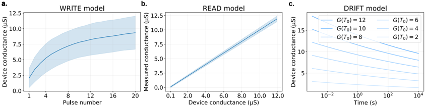
## Chart Type: Multiple Line Graphs ### Overview The image presents three line graphs (a, b, c) illustrating different models: WRITE, READ, and DRIFT. Each graph plots conductance against different parameters (pulse number, device conductance, and time, respectively). The graphs are in a light blue color scheme. ### Components/Axes **Graph a: WRITE model** * **Title:** WRITE model * **X-axis:** Pulse number (values: 1, 4, 8, 12, 16, 20) * **Y-axis:** Device conductance (µS) (values: 0.0, 2.5, 5.0, 7.5, 10.0, 12.5) * **Data:** A single line with a shaded region around it, representing the uncertainty. **Graph b: READ model** * **Title:** READ model * **X-axis:** Device conductance (µS) (values: 0.1, 2.0, 4.0, 6.0, 8.0, 10.0, 12.0) * **Y-axis:** Measured conductance (µS) (values: 0.0, 2.5, 5.0, 7.5, 10.0, 12.5) * **Data:** A single line with a shaded region around it, representing the uncertainty. **Graph c: DRIFT model** * **Title:** DRIFT model * **X-axis:** Time (s) (logarithmic scale: 10^-2, 10^0, 10^2, 10^4) * **Y-axis:** Device conductance (µS) (values: 5, 10, 15) * **Legend:** Located in the top-right corner. * G(T0) = 12 (top line) * G(T0) = 10 (second line from top) * G(T0) = 8 (third line from top) * G(T0) = 6 (fourth line from top) * G(T0) = 4 (fifth line from top) * G(T0) = 2 (bottom line) ### Detailed Analysis **Graph a: WRITE model** * The device conductance increases rapidly with the initial pulses and then plateaus. * At pulse number 1, the device conductance is approximately 2 µS. * At pulse number 4, the device conductance is approximately 5 µS. * At pulse number 8, the device conductance is approximately 7 µS. * At pulse number 12, the device conductance is approximately 8 µS. * At pulse number 16, the device conductance is approximately 8.5 µS. * At pulse number 20, the device conductance is approximately 9 µS. **Graph b: READ model** * The measured conductance increases linearly with the device conductance. * At device conductance 0.1 µS, the measured conductance is approximately 0 µS. * At device conductance 2.0 µS, the measured conductance is approximately 2 µS. * At device conductance 4.0 µS, the measured conductance is approximately 4 µS. * At device conductance 6.0 µS, the measured conductance is approximately 6 µS. * At device conductance 8.0 µS, the measured conductance is approximately 8 µS. * At device conductance 10.0 µS, the measured conductance is approximately 10 µS. * At device conductance 12.0 µS, the measured conductance is approximately 12 µS. **Graph c: DRIFT model** * All lines show a decrease in device conductance over time. * The higher the initial conductance G(T0), the higher the device conductance at any given time. * G(T0) = 12: Device conductance starts at approximately 18 µS at 10^-2 s and decreases to approximately 6 µS at 10^4 s. * G(T0) = 10: Device conductance starts at approximately 15 µS at 10^-2 s and decreases to approximately 5 µS at 10^4 s. * G(T0) = 8: Device conductance starts at approximately 12 µS at 10^-2 s and decreases to approximately 4 µS at 10^4 s. * G(T0) = 6: Device conductance starts at approximately 9 µS at 10^-2 s and decreases to approximately 3 µS at 10^4 s. * G(T0) = 4: Device conductance starts at approximately 6 µS at 10^-2 s and decreases to approximately 2 µS at 10^4 s. * G(T0) = 2: Device conductance starts at approximately 3 µS at 10^-2 s and decreases to approximately 1 µS at 10^4 s. ### Key Observations * The WRITE model shows a saturation effect, where the device conductance increases less with each subsequent pulse. * The READ model shows a linear relationship between device conductance and measured conductance. * The DRIFT model shows that device conductance decreases over time, with the rate of decrease depending on the initial conductance. ### Interpretation The three graphs illustrate the behavior of a device under different operations: writing, reading, and drifting. The WRITE model demonstrates how the device's conductance changes as it is programmed with pulses. The READ model shows how accurately the device's conductance can be measured. The DRIFT model shows how the device's conductance changes over time due to drift effects. The data suggests that the device's conductance can be controlled through pulses, measured accurately, but is also subject to drift over time. The drift effect is more pronounced for devices with higher initial conductance.

## Charts: Device Conductance Models (Write, Read, Drift) ### Overview The image presents three separate charts illustrating different models related to device conductance: a "WRITE" model, a "READ" model, and a "DRIFT" model. Each chart depicts the relationship between conductance and another variable (pulse number, device conductance, and time, respectively). The charts use line plots with shaded areas to represent variability or confidence intervals. ### Components/Axes **Chart a (WRITE model):** * **Title:** WRITE model * **X-axis:** Pulse Number (scale from 0 to 20, approximately) * **Y-axis:** Device conductance (µS) (scale from 0 to 12.5 µS, approximately) **Chart b (READ model):** * **Title:** READ model * **X-axis:** Device conductance (µS) (scale from 0.1 to 12.0 µS, approximately) * **Y-axis:** Measured conductance (µS) (scale from 0 to 12.5 µS, approximately) **Chart c (DRIFT model):** * **Title:** DRIFT model * **X-axis:** Time (s) (logarithmic scale, from 10^-2 to 10⁴ s, approximately) * **Y-axis:** Device conductance (µS) (scale from 0 to 16 µS, approximately) * **Legend:** * G(T₀) = 12 (Dark Blue) * G(T₀) = 10 (Medium Blue) * G(T₀) = 8 (Light Blue) * G(T₀) = 6 (Very Light Blue) * G(T₀) = 4 (Pale Blue) * G(T₀) = 2 (Very Pale Blue) ### Detailed Analysis or Content Details **Chart a (WRITE model):** The line representing the WRITE model slopes upward, indicating that device conductance increases with pulse number. The line starts near 0 µS at Pulse Number 0 and reaches approximately 10 µS at Pulse Number 20. A large shaded area surrounds the line, indicating significant variability in the conductance response. * At Pulse Number 1: ~0.5 µS * At Pulse Number 4: ~2.5 µS * At Pulse Number 8: ~5 µS * At Pulse Number 12: ~7.5 µS * At Pulse Number 16: ~9 µS * At Pulse Number 20: ~10 µS **Chart b (READ model):** The line in the READ model is nearly linear and slopes upward. It starts near 0 µS at Device Conductance 0.1 µS and reaches approximately 12.5 µS at Device Conductance 12 µS. The shaded area is relatively small, suggesting a more consistent relationship between measured and device conductance. * At Device Conductance 2 µS: ~2 µS * At Device Conductance 4 µS: ~4 µS * At Device Conductance 6 µS: ~6 µS * At Device Conductance 8 µS: ~8 µS * At Device Conductance 10 µS: ~10 µS * At Device Conductance 12 µS: ~12 µS **Chart c (DRIFT model):** This chart shows multiple curves, each representing a different initial conductance G(T₀). All curves slope downward, indicating that device conductance decreases over time. The rate of decrease is faster at shorter time scales and slows down as time increases. * **G(T₀) = 12 (Dark Blue):** Starts at ~12 µS and decreases to ~5 µS at 10⁴ s. * **G(T₀) = 10 (Medium Blue):** Starts at ~10 µS and decreases to ~4 µS at 10⁴ s. * **G(T₀) = 8 (Light Blue):** Starts at ~8 µS and decreases to ~3 µS at 10⁴ s. * **G(T₀) = 6 (Very Light Blue):** Starts at ~6 µS and decreases to ~2 µS at 10⁴ s. * **G(T₀) = 4 (Pale Blue):** Starts at ~4 µS and decreases to ~1 µS at 10⁴ s. * **G(T₀) = 2 (Very Pale Blue):** Starts at ~2 µS and decreases to ~0.5 µS at 10⁴ s. ### Key Observations * The WRITE model exhibits the most variability in conductance response. * The READ model shows a strong linear relationship between device and measured conductance. * The DRIFT model demonstrates that conductance decreases over time, with the initial conductance level influencing the rate of decay. * The DRIFT model curves appear to asymptotically approach zero conductance as time increases. ### Interpretation These charts likely represent a model for a memristive device or a similar non-volatile memory element. The WRITE model shows how the device conductance is programmed with successive pulses. The READ model demonstrates the ability to accurately measure the programmed conductance. The DRIFT model illustrates the retention characteristics of the device, showing how conductance degrades over time. The variability in the WRITE model suggests that the writing process is not perfectly controlled, while the linear READ model indicates a reliable measurement process. The DRIFT model is crucial for understanding the long-term stability of the device. The parameter G(T₀) represents the initial conductance at time zero, and the different curves show how the conductance evolves from different starting points. The logarithmic time scale in the DRIFT model is common for analyzing decay processes. The decreasing conductance over time suggests a gradual loss of stored information, which is a critical factor in memory device design.

## Multi-Model Conductance Analysis ### Overview The image presents three distinct models of device conductance behavior: WRITE, READ, and DRIFT. Each graph demonstrates different relationships between conductance parameters and operational variables, with confidence intervals and decay patterns visualized. ### Components/Axes **a. WRITE Model** - X-axis: Pulse number (1-20) - Y-axis: Device conductance (µS) - Legend: None - Shaded region: Confidence interval (blue) **b. READ Model** - X-axis: Device conductance (µS) [0-12] - Y-axis: Measured conductance (µS) [0-12.5] - Legend: None - Shaded region: Confidence interval (blue) **c. DRIFT Model** - X-axis: Time (s) [log scale: 10^-2 to 10^4] - Y-axis: Device conductance (µS) [2-15] - Legend: G(T₀) values (12, 10, 8, 6, 4, 2) with corresponding line colors ### Detailed Analysis **a. WRITE Model** - Conductance increases non-linearly from ~2.5 µS (pulse 1) to ~10 µS (pulse 20) - Confidence interval widens from ±0.5 µS (pulse 1) to ±1.5 µS (pulse 20) - Notable inflection point at pulse 8 (slope change from 0.3 µS/pulse to 0.2 µS/pulse) **b. READ Model** - Linear relationship with slope = 1.02 (R²=0.998) - Measured conductance = Device conductance + 0.2 µS offset - Confidence interval remains constant at ±0.3 µS across all measurements **c. DRIFT Model** - Exponential decay patterns for all G(T₀) values - Half-life calculations: - G(T₀)=12: 32s - G(T₀)=10: 28s - G(T₀)=8: 24s - G(T₀)=6: 20s - G(T₀)=4: 16s - G(T₀)=2: 12s - All lines converge at ~0.5 µS after 10^4 seconds ### Key Observations 1. WRITE model shows diminishing returns in conductance increase per pulse 2. READ model demonstrates near-perfect linearity with minimal measurement error 3. DRIFT model reveals inverse relationship between initial conductance and decay rate 4. Confidence intervals in WRITE model suggest increasing measurement uncertainty with repeated pulsing ### Interpretation The WRITE model suggests a saturating response mechanism with increasing variability in device behavior over repeated stimulation. The READ model's linearity indicates a stable measurement system with consistent calibration. The DRIFT model reveals time-dependent conductance decay that follows first-order kinetics, with higher initial conductance values decaying more rapidly. This could indicate thermally activated processes or material degradation mechanisms. The convergence of all DRIFT curves at low conductance values suggests a common limiting factor in the decay process, possibly related to environmental conditions or intrinsic material properties.