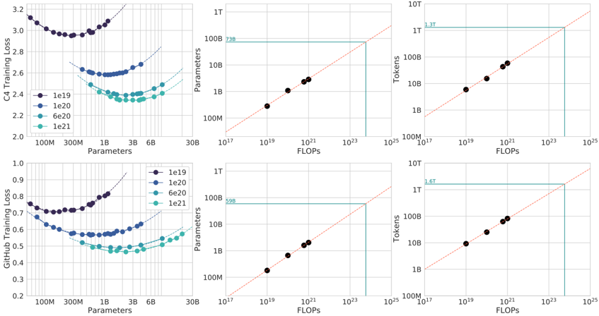
\n ## Multi-Panel Scaling Law Charts: C4 and GitHub Training Loss ### Overview The image contains six charts arranged in a 2x3 grid. The top row analyzes "C4 Training Loss," and the bottom row analyzes "GitHub Training Loss." Each row contains three related plots that explore the relationship between model parameters, compute (FLOPs), training tokens, and loss. The charts are technical plots typical of machine learning scaling law research, using logarithmic scales and scatter plots with trend lines. ### Components/Axes **General Layout:** - **Top Row (C4):** Three charts horizontally aligned. - **Bottom Row (GitHub):** Three charts horizontally aligned. - **Common Elements:** All charts have a white background with light gray grid lines. Data points are colored circles. Dashed orange lines represent power-law trend fits. **Chart-Specific Components:** 1. **Top-Left & Bottom-Left Charts (Loss vs. Parameters):** * **X-axis:** "Parameters" (log scale). Ticks: 100M, 300M, 1B, 3B, 6B, 30B. * **Y-axis:** "C4 Training Loss" (top) / "GitHub Training Loss" (bottom). Linear scale. * **Legend:** Located in the top-right corner of each chart. Four series labeled by token count: * `1e19` (Dark Purple) * `1e20` (Medium Blue) * `6e20` (Teal) * `1e21` (Light Teal) * **Data:** Four distinct U-shaped curves, one per token count series. 2. **Top-Middle & Bottom-Middle Charts (Parameters vs. FLOPs):** * **X-axis:** "FLOPs" (log scale). Ticks: 10¹⁷, 10¹⁹, 10²¹, 10²³, 10²⁵. * **Y-axis:** "Parameters" (log scale). Ticks: 100M, 1B, 10B, 100B, 1T. * **Horizontal Line:** A solid teal line marks a specific parameter count. * Top Chart: Labeled "73B" at the line's left end. * Bottom Chart: Labeled "99B" at the line's left end. * **Data:** A set of dark purple data points following a diagonal trend line. 3. **Top-Right & Bottom-Right Charts (Tokens vs. FLOPs):** * **X-axis:** "FLOPs" (log scale). Same as middle charts. * **Y-axis:** "Tokens" (log scale). Ticks: 100M, 1B, 10B, 100B, 1T, 10T. * **Horizontal Line:** A solid teal line marks a specific token count. * Top Chart: Labeled "1.3T" at the line's left end. * Bottom Chart: Labeled "1.6T" at the line's left end. * **Data:** A set of dark purple data points following a diagonal trend line. ### Detailed Analysis **1. C4 Training Loss (Top Row)** * **Loss vs. Parameters (Top-Left):** * **Trend:** Each token series forms a U-shaped curve. Loss initially decreases as parameters increase, reaches a minimum, and then increases. * **Data Points (Approximate):** * `1e19` (Dark Purple): Minimum loss ~2.95 at ~300M parameters. * `1e20` (Medium Blue): Minimum loss ~2.6 at ~1B parameters. * `6e20` (Teal): Minimum loss ~2.4 at ~3B parameters. * `1e21` (Light Teal): Minimum loss ~2.35 at ~6B parameters. * **Observation:** More training tokens shift the optimal parameter count (minimum of the U-curve) to the right and lower the achievable minimum loss. * **Parameters vs. FLOPs (Top-Middle):** * **Trend:** A strong positive linear relationship on a log-log scale (power law). More FLOPs correlate with more parameters. * **Data Points:** Five dark purple points lie almost perfectly on the dashed orange trend line. * **Key Value:** The horizontal line indicates a model size of **73B parameters** corresponds to approximately **10²⁴ FLOPs**. * **Tokens vs. FLOPs (Top-Right):** * **Trend:** A strong positive linear relationship on a log-log scale. * **Data Points:** Five dark purple points lie on the dashed orange trend line. * **Key Value:** The horizontal line indicates **1.3T tokens** corresponds to approximately **10²⁴ FLOPs**. **2. GitHub Training Loss (Bottom Row)** * **Loss vs. Parameters (Bottom-Left):** * **Trend:** Similar U-shaped curves as the C4 chart, but with lower absolute loss values. * **Data Points (Approximate):** * `1e19` (Dark Purple): Minimum loss ~0.72 at ~300M parameters. * `1e20` (Medium Blue): Minimum loss ~0.58 at ~1B parameters. * `6e20` (Teal): Minimum loss ~0.5 at ~3B parameters. * `1e21` (Light Teal): Minimum loss ~0.48 at ~6B parameters. * **Observation:** The same scaling pattern holds: more tokens allow for larger optimal models and lower loss. * **Parameters vs. FLOPs (Bottom-Middle):** * **Trend:** Identical positive power-law relationship as the C4 chart. * **Key Value:** The horizontal line indicates a model size of **99B parameters** corresponds to approximately **10²⁴ FLOPs**. * **Tokens vs. FLOPs (Bottom-Right):** * **Trend:** Identical positive power-law relationship as the C4 chart. * **Key Value:** The horizontal line indicates **1.6T tokens** corresponds to approximately **10²⁴ FLOPs**. ### Key Observations 1. **Consistent Scaling Laws:** The relationship between Parameters, FLOPs, and Tokens follows a consistent power law across both datasets (C4 and GitHub), as shown by the linear trends on log-log plots. 2. **Optimal Model Size:** For a fixed token budget, there exists an optimal model size (parameter count) that minimizes training loss. Using more parameters than this optimum leads to increased loss (overfitting). 3. **Dataset Difference:** Models trained on GitHub data achieve significantly lower loss values (~0.5-0.7) compared to models trained on C4 data (~2.4-3.0) for similar parameter counts and token budgets. 4. **Compute Allocation:** At a fixed compute budget of ~10²⁴ FLOPs, the charts suggest different optimal allocations: for C4, ~73B parameters trained on ~1.3T tokens; for GitHub, ~99B parameters trained on ~1.6T tokens. ### Interpretation These charts empirically demonstrate **scaling laws** for neural language models. They show that model performance (training loss) is predictable based on three key resources: model size (parameters), dataset size (tokens), and compute budget (FLOPs). The U-shaped curves in the loss vs. parameter plots are critical. They illustrate the **bias-variance tradeoff** in a scaling context. For a given dataset size (token count), a model that is too small is underfit (high bias), while a model that is too large is overfit (high variance). The minimum of the curve represents the optimal model capacity for that data volume. The power-law relationships in the middle and right charts are the foundation for **compute-optimal training**. They allow researchers to predict, for a given total FLOPs budget, what combination of model parameters and training tokens will yield the best performance. The difference in optimal points between C4 and GitHub (73B/1.3T vs. 99B/1.6T) suggests that the optimal allocation is **data-dependent**; the GitHub dataset may be larger or of a different nature that benefits from a slightly larger model trained on more tokens for the same compute cost. In essence, this image provides a quantitative framework for making strategic decisions in large language model training: how to allocate a fixed compute budget between making a model bigger and training it on more data to achieve the lowest possible loss.