## Comparative Line Charts: HMC Convergence Behavior
### Overview
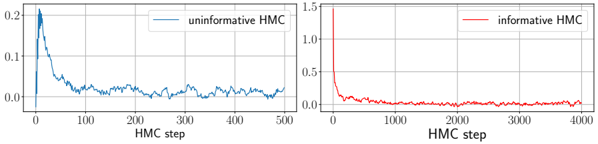
The image displays two side-by-side line charts comparing the performance of two Hamiltonian Monte Carlo (HMC) sampling methods over different numbers of steps. The left chart shows the "uninformative HMC" method, and the right chart shows the "informative HMC" method. Both charts plot a metric (likely an error, divergence, or autocorrelation measure) on the y-axis against the number of HMC steps on the x-axis.
### Components/Axes
**Left Chart:**
* **Title/Label:** None visible.
* **X-axis:** Label: "HMC step". Scale: Linear, from 0 to 500, with major ticks at 0, 100, 200, 300, 400, 500.
* **Y-axis:** No explicit label. Scale: Linear, from 0.0 to 0.2, with major ticks at 0.0, 0.1, 0.2.
* **Legend:** Located in the top-right corner. Contains a single entry: a blue line labeled "uninformative HMC".
**Right Chart:**
* **Title/Label:** None visible.
* **X-axis:** Label: "HMC step". Scale: Linear, from 0 to 4000, with major ticks at 0, 1000, 2000, 3000, 4000.
* **Y-axis:** No explicit label. Scale: Linear, from 0.0 to 1.5, with major ticks at 0.0, 0.5, 1.0, 1.5.
* **Legend:** Located in the top-right corner. Contains a single entry: a red line labeled "informative HMC".
### Detailed Analysis
**Left Chart (Uninformative HMC - Blue Line):**
* **Trend Verification:** The blue line exhibits a sharp initial drop followed by a noisy, gradually decaying oscillation. The overall trend is downward, but with significant variance.
* **Data Points (Approximate):**
* At step 0: y ≈ 0.2 (starting point).
* At step ~10: y drops sharply to a minimum near 0.0.
* At step ~20: y spikes back up to a peak near 0.2.
* From step ~20 to 500: The line fluctuates noisily between approximately 0.0 and 0.08, with a very gradual downward trend. By step 500, the value is approximately 0.02.
**Right Chart (Informative HMC - Red Line):**
* **Trend Verification:** The red line shows an extremely rapid initial decay, followed by a long, flat tail very close to zero with minimal noise.
* **Data Points (Approximate):**
* At step 0: y ≈ 1.5 (starting point, much higher than the left chart).
* At step ~100: y has decayed rapidly to below 0.1.
* From step ~200 to 4000: The line remains very close to y=0.0, fluctuating minimally (estimated range 0.0 to 0.03). The value appears stable and near zero for the vast majority of the steps shown.
### Key Observations
1. **Scale Difference:** The y-axis scales differ significantly (max 0.2 vs. max 1.5), indicating the "informative HMC" starts from a much higher initial value or error.
2. **Convergence Speed:** The "informative HMC" (right) converges to a near-zero value much faster in terms of absolute steps (within ~200 steps) compared to the "uninformative HMC" (left), which is still fluctuating significantly at step 500.
3. **Stability/Noise:** The "uninformative HMC" signal is persistently noisy throughout the 500 steps. The "informative HMC" signal becomes extremely stable and low-noise after its initial rapid descent.
4. **X-axis Range:** The right chart plots 8 times more steps (4000 vs. 500), suggesting the "informative" method is being evaluated over a longer horizon, yet it maintains its stable, low value.
### Interpretation
The charts demonstrate a clear performance comparison between two HMC sampling strategies. The "informative HMC" method, likely initialized with better prior information or a more efficient proposal mechanism, shows superior convergence properties. It rapidly reduces the measured metric (e.g., distance from a target distribution, energy error) from a high initial value and then maintains a stable, low-error state. This suggests it is both efficient and reliable for sampling.
In contrast, the "uninformative HMC" method struggles. It starts from a lower initial value but fails to converge cleanly, exhibiting persistent high-frequency noise and a much slower decay rate. This indicates inefficient exploration of the parameter space, potentially due to poor tuning or lack of guiding information, leading to higher autocorrelation and less reliable samples within the observed timeframe.
The key takeaway is that incorporating "information" (e.g., through better preconditioning, informed initialization, or adaptive tuning) into the HMC algorithm dramatically improves its convergence speed and the stability of the resulting chain, which is critical for efficient Bayesian computation. The "uninformative" approach would require many more steps to achieve the same level of stability, if it can achieve it at all.