\n
## Line Chart: Per-Period Regret Over Time for Two Thompson Sampling Agents
### Overview
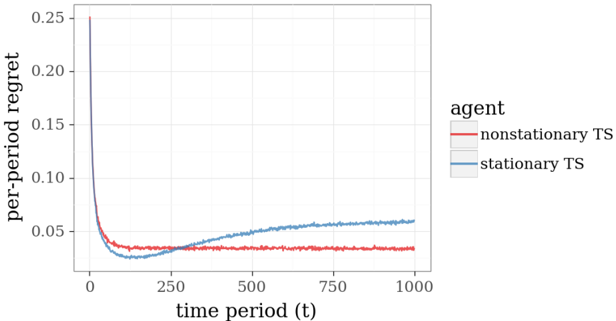
The image displays a line chart comparing the performance of two algorithms, labeled as "agents," over 1000 time periods. The performance metric is "per-period regret," where a lower value indicates better performance. The chart shows that one agent maintains a consistently low regret after an initial learning phase, while the other's performance degrades over time.
### Components/Axes
* **Chart Type:** Line chart with two data series.
* **Y-Axis:**
* **Label:** `per-period regret`
* **Scale:** Linear, ranging from 0.00 to 0.25.
* **Major Tick Marks:** 0.00, 0.05, 0.10, 0.15, 0.20, 0.25.
* **X-Axis:**
* **Label:** `time period (t)`
* **Scale:** Linear, ranging from 0 to 1000.
* **Major Tick Marks:** 0, 250, 500, 750, 1000.
* **Legend:**
* **Position:** Centered on the right side of the plot area.
* **Title:** `agent`
* **Series 1:** `nonstationary TS` - Represented by a **red line**.
* **Series 2:** `stationary TS` - Represented by a **blue line**.
### Detailed Analysis
**1. Nonstationary TS (Red Line):**
* **Trend Verification:** The line exhibits a very steep, near-vertical descent from a high initial value, followed by a sharp knee, and then transitions to a nearly flat, stable plateau with minor fluctuations.
* **Data Points (Approximate):**
* At `t ≈ 0`: Regret starts at or above the maximum y-axis value of **0.25**.
* At `t ≈ 50`: Regret drops dramatically to approximately **0.04**.
* From `t ≈ 100 to t = 1000`: Regret stabilizes and fluctuates within a narrow band between approximately **0.03 and 0.04**. The line shows no significant upward or downward trend in this long-term phase.
**2. Stationary TS (Blue Line):**
* **Trend Verification:** The line also shows a steep initial descent, but its minimum is reached later than the red line. After reaching its minimum, it begins a slow, steady, and persistent upward slope for the remainder of the time periods.
* **Data Points (Approximate):**
* At `t ≈ 0`: Regret starts at or above **0.25**.
* At `t ≈ 100`: Reaches its minimum regret of approximately **0.025**.
* **Crossover Point:** At approximately `t = 250`, the blue line crosses above the red line and remains above it for all subsequent time periods.
* At `t = 500`: Regret has risen to approximately **0.05**.
* At `t = 1000`: Regret ends at its highest point since the initial drop, approximately **0.06**.
### Key Observations
1. **Initial Learning Phase:** Both agents start with very high regret and learn rapidly, reducing regret by over 80% within the first 100 time periods.
2. **Performance Divergence:** A critical divergence occurs around `t = 250`. The `nonstationary TS` agent maintains its low regret, while the `stationary TS` agent's performance begins to degrade steadily.
3. **Long-Term Performance:** By the end of the observed period (`t = 1000`), the `nonstationary TS` agent's regret is roughly **33% lower** than that of the `stationary TS` agent (approx. 0.04 vs. 0.06).
4. **Stability vs. Drift:** The red line (`nonstationary TS`) is characterized by long-term stability after learning. The blue line (`stationary TS`) is characterized by a continuous, positive drift (increasing regret) after its initial learning phase.
### Interpretation
This chart likely illustrates a comparison between two variants of the Thompson Sampling (TS) algorithm in a **non-stationary bandit environment**—a scenario where the underlying probabilities of rewards from different options change over time.
* The `nonstationary TS` agent is designed to detect and adapt to such changes. Its stable, low regret suggests it successfully tracks the changing environment, continuously adjusting its strategy to minimize loss.
* The `stationary TS` agent assumes the environment is fixed. Its initial low regret shows it learned the *initial* state well. However, its steadily increasing regret after `t=250` is a classic signature of **concept drift**. The agent's model becomes outdated as the environment changes, leading to increasingly poor decisions and higher regret.
* The **crossover point** is the most critical feature. It marks the moment when the environmental changes have accumulated enough to make the adaptive (`nonstationary`) strategy definitively superior to the static (`stationary`) one. This visualizes the fundamental cost of failing to account for non-stationarity in dynamic systems.
**In summary, the data demonstrates the significant long-term advantage of using an algorithm capable of adaptation (`nonstationary TS`) over one that assumes a static environment (`stationary TS`) when operating in a changing world.** The `stationary TS` agent is not "bad"—it simply solves the wrong problem after the environment shifts.