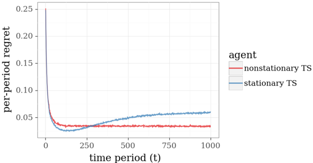
## Line Graph: Per-Period Regret Over Time for Two Agents
### Overview
The graph illustrates the per-period regret of two agents—nonstationary TS (red line) and stationary TS (blue line)—over 1,000 time periods. Both agents exhibit a sharp initial decline in regret, followed by stabilization at distinct plateau levels.
### Components/Axes
- **X-axis**: "time period (t)" with markers at 0, 250, 500, 750, and 1,000.
- **Y-axis**: "per-period regret" scaled from 0 to 0.25 in increments of 0.05.
- **Legend**: Located in the top-right corner, associating:
- **Red line**: Nonstationary TS
- **Blue line**: Stationary TS
### Detailed Analysis
1. **Nonstationary TS (Red Line)**:
- Starts at ~0.25 regret at time 0.
- Drops sharply to ~0.04 by time 250.
- Remains flat at ~0.04 for the remainder of the time periods (500–1,000).
2. **Stationary TS (Blue Line)**:
- Starts at ~0.25 regret at time 0.
- Declines gradually, reaching ~0.05 by time 500.
- Plateaus at ~0.05 for the remainder of the time periods (500–1,000).
### Key Observations
- Both agents show a rapid initial reduction in regret, but the nonstationary TS stabilizes significantly faster (~250 time periods vs. ~500 for stationary TS).
- The nonstationary TS achieves a lower asymptotic regret (~0.04 vs. ~0.05 for stationary TS).
- No anomalies or outliers are observed; trends are smooth and consistent.
### Interpretation
The data suggests that the nonstationary TS agent adapts more efficiently to changing conditions, achieving lower regret faster than the stationary TS. The stationary TS’s slower convergence and higher plateau regret imply reduced adaptability, possibly due to fixed parameters. The plateau values indicate that both agents eventually reach a steady state, but the nonstationary TS demonstrates superior long-term performance in minimizing regret. This aligns with theoretical expectations for nonstationary algorithms in dynamic environments.