## Diagram: Graph Neural Network Pipeline for Human Pose Estimation
### Overview
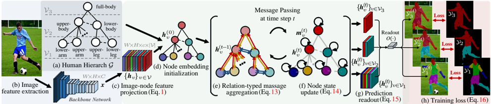
The image illustrates a multi-stage pipeline for a graph neural network (GNN) model designed for human pose estimation or a similar structured prediction task from an input image. The process flows from left to right, starting with an image of a person, extracting features, constructing a hierarchical graph representing the human body, processing this graph through node embedding and message-passing layers, and finally generating predictions with associated losses for training.
### Components/Axes
The diagram is segmented into eight labeled components, (a) through (h), connected by arrows indicating data flow.
* **(a) Human Hierarchy G**: A tree-structured graph representing the human body. It has three hierarchical levels:
* **V3 (Top Level)**: A single node labeled `full-body`.
* **V2 (Middle Level)**: Two nodes labeled `upper-body` and `lower-body`.
* **V1 (Bottom Level)**: Four nodes labeled `lower-arm`, `upper-arm`, `upper-leg`, and `lower-leg`.
* Lines connect parent nodes to their child nodes, showing the hierarchical relationship.
* **(b) Image feature extraction**: An input image of a person playing soccer is processed by a "Backbone Network" (depicted as a convolutional neural network) to produce a feature map `x` with dimensions `W x H x C`.
* **(c) Image-node feature projection (Eq. 1)**: The feature map `x` is projected to create initial node features `{h_v}` for each node `v` in the graph. This is represented as a 3D tensor of size `W x H x (|V| * M)`, where `|V|` is the number of nodes and `M` is the feature dimension per node.
* **(d) Node embedding initialization**: The projected features are used to initialize the state `h_v^(0)` for each node in the graph. The nodes are color-coded (red, blue, green, yellow, purple, cyan, orange).
* **(e) Relation-typed message aggregation (Eq. 13)**: This is the core message-passing step at time step `t`. It shows a graph where nodes exchange information. Arrows indicate messages being sent between connected nodes. The equation `h_v^(t-1)` suggests the node state from the previous step is used. The label `m_v^(t)` likely represents the aggregated message for node `v` at step `t`.
* **(f) Node state update (Eq. 14)**: The aggregated message is used to update the node's state to `h_v^(t)`. The diagram shows the same graph structure with updated node states.
* **(g) Prediction readout (Eq. 15)**: The final node states `{h_v^(t)}` for nodes in levels `V3`, `V2`, and `V1` are passed through a readout function `O(·)` to generate predictions. The predictions are visualized as colored segmentation masks or heatmaps overlaid on the original image, corresponding to different body parts (full-body, upper-body, lower-body, etc.).
* **(h) Training loss (Eq. 16)**: The predictions from different hierarchy levels (`V3`, `V2`, `V1`) are compared against ground truth data (shown as black silhouettes with colored body parts) to compute a `Loss` for each level. This indicates a multi-scale or hierarchical training objective.
### Detailed Analysis
The pipeline describes a **Graph-based Human Pose Estimation** method.
1. **Input**: An RGB image.
2. **Feature Extraction**: A standard CNN backbone extracts a dense feature map.
3. **Graph Construction**: A predefined hierarchical graph `G` models the human body structure. The feature map is projected to initialize features for each node in this graph.
4. **Graph Processing**: A Graph Neural Network operates on this hierarchy. It performs iterative **message passing** (Eq. 13) and **node state updates** (Eq. 14). The term "Relation-typed" suggests different types of messages may be passed along different edges (e.g., parent-child vs. sibling connections).
5. **Multi-level Prediction**: Readout functions (Eq. 15) generate predictions from node states at *all three levels* of the hierarchy (`V1`, `V2`, `V3`). This suggests the model makes predictions for the whole body, major body sections, and individual limbs simultaneously.
6. **Hierarchical Supervision**: The training loss (Eq. 16) is computed separately for predictions at each hierarchy level, providing direct supervision to intermediate representations and likely improving gradient flow and model interpretability.
### Key Observations
* The model explicitly encodes **anatomical priors** through the hierarchical graph `G`.
* It employs **deep supervision** by calculating losses at multiple graph levels (`V1`, `V2`, `V3`).
* The process is **end-to-end differentiable**, from image input to final loss computation.
* The visualization in (g) and (h) suggests the output is a **part segmentation** or **part affinity field** map, not just a set of keypoint coordinates.
### Interpretation
This diagram represents a sophisticated approach to human pose estimation that moves beyond simple keypoint regression. By framing the problem as **message passing on a structured graph**, the model can explicitly reason about the spatial and semantic relationships between body parts. The hierarchical design (`full-body` -> `upper/lower-body` -> `limbs`) mirrors how humans perceive pose, potentially leading to more robust predictions, especially in cases of occlusion or unusual poses. The multi-level supervision ensures that the model learns meaningful representations at each stage of abstraction, from coarse body sections to fine-grained limbs. This architecture is characteristic of modern Graph Neural Network (GNN) applications in computer vision, where relational inductive biases are injected into deep learning models to handle structured data like the human body.