## Diagram: Automated Math Problem Solving Pipeline with Self-Correction
### Overview
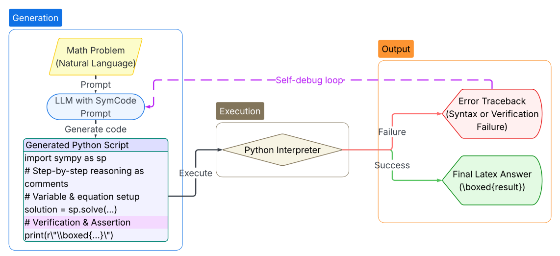
The image is a flowchart illustrating a system that uses a Large Language Model (LLM) to generate and execute Python code for solving math problems, incorporating a self-debugging loop for error correction. The process flows from a natural language problem input to a final formatted answer, with distinct phases for generation, execution, and output handling.
### Components/Axes
The diagram is organized into three primary, color-coded regions:
1. **Generation (Blue Box, Left):** Contains the problem input, the LLM processing unit, and the generated code output.
2. **Execution (Brown Box, Center):** Contains the Python interpreter that runs the generated code.
3. **Output (Orange Box, Right):** Contains the two possible final states: an error report or the final answer.
**Key Components & Labels:**
* **Math Problem (Natural Language):** Yellow parallelogram. The starting input.
* **LLM with SymCode Prompt:** Blue oval. The core processing unit that receives the problem prompt.
* **Generated Python Script:** Purple rectangle. Contains a code snippet with the following transcribed text:
```
import sympy as sp
# Step-by-step reasoning as comments
# Variable & equation setup
solution = sp.solve(...)
# Verification & Assertion
print(r"\boxed{...}")
```
* **Python Interpreter:** Beige diamond shape. The execution engine.
* **Error Traceback (Syntax or Verification Failure):** Red hexagon. The failure output state.
* **Final Latex Answer (\boxed{result}):** Green hexagon. The successful output state.
* **Self-debug loop:** A dashed purple line connecting the "Error Traceback" back to the "LLM with SymCode Prompt".
**Flow & Connections:**
* A solid black arrow labeled "Prompt" connects the "Math Problem" to the "LLM".
* A solid black arrow labeled "Generate code" connects the "LLM" to the "Generated Python Script".
* A solid black arrow labeled "Execute" connects the "Generated Python Script" to the "Python Interpreter".
* From the "Python Interpreter", two paths diverge:
* A red arrow labeled "Failure" leads to the "Error Traceback".
* A green arrow labeled "Success" leads to the "Final Latex Answer".
* The "Self-debug loop" (dashed purple line) originates from the "Error Traceback" and feeds back into the "LLM with SymCode Prompt", creating a corrective cycle.
### Detailed Analysis
The process is a sequential pipeline with a conditional branch and a feedback loop.
1. **Input Stage:** A math problem posed in natural language is provided.
2. **Generation Stage:** An LLM, prompted with "SymCode" (suggesting a focus on symbolic mathematics), generates a Python script. The script template uses the `sympy` library, includes step-by-step reasoning as comments, sets up variables and equations, solves them, performs verification, and prints the result in a LaTeX `\boxed{}` format.
3. **Execution Stage:** The generated script is passed to a Python interpreter.
4. **Output Stage (Conditional):**
* **On Success:** The interpreter produces a "Final Latex Answer" formatted as `\boxed{result}`.
* **On Failure:** The interpreter produces an "Error Traceback" indicating either a syntax error in the generated code or a verification failure (e.g., an assertion check within the code failed).
5. **Correction Mechanism:** The "Self-debug loop" is activated upon failure. The error traceback is sent back to the LLM, presumably to inform a revised code generation attempt, creating an iterative refinement process.
### Key Observations
* **Hybrid Reasoning:** The system combines neural (LLM) and symbolic (Python/SymPy) approaches. The LLM handles the translation from language to code, while the symbolic solver handles the precise mathematical computation.
* **Built-in Verification:** The code template includes a "Verification & Assertion" step, indicating the system is designed to check its own work before outputting a final answer.
* **Error-Driven Iteration:** The architecture explicitly accounts for failure modes (syntax, verification) and includes a dedicated feedback path for autonomous correction, moving beyond a simple one-shot generation pipeline.
* **Structured Output:** The final answer is constrained to a specific LaTeX format (`\boxed{}`), facilitating easy extraction and presentation.
### Interpretation
This diagram represents a robust architecture for automated mathematical problem-solving. It addresses key limitations of pure LLM approaches (hallucination, computational inaccuracy) by grounding the solution in executable, verifiable code. The "SymCode Prompt" suggests specialized training or prompting to improve code generation for mathematical tasks.
The **self-debug loop is the most critical component** from a systems perspective. It transforms the pipeline from a fragile, open-loop system into a more resilient, closed-loop one. The system can potentially recover from its own mistakes, mimicking a human programmer's debug cycle. This increases reliability and reduces the need for human intervention.
The clear separation of **Generation, Execution, and Output** reflects good software design principles, isolating different types of failures (e.g., a generation error vs. a runtime error). The use of distinct colors and shapes for each component type (parallelogram for I/O, oval for process, diamond for decision, hexagon for terminal state) follows standard flowchart conventions, making the logic easy to follow.
In essence, the image depicts not just a tool for solving math problems, but a framework for building more reliable and self-correcting AI agents that combine large language models with traditional software engineering practices.