## [Log-Log Scatter Plot with Linear Fits]: Scaling of Monte Carlo Stops vs. Dimension
### Overview
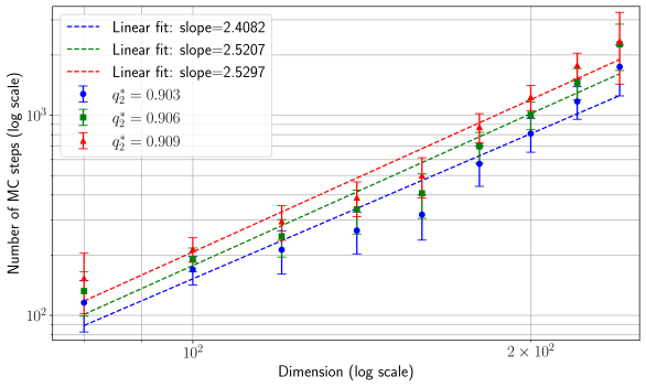
The image is a scientific log-log plot showing the relationship between the dimension of a problem (x-axis) and the number of Monte Carlo (MC) stops required (y-axis). Three distinct data series are plotted, each with error bars and a corresponding linear fit line. The plot demonstrates a power-law relationship between the variables.
### Components/Axes
* **Chart Type:** Scatter plot with error bars and linear regression lines on a log-log scale.
* **X-Axis:**
* **Label:** `Dimension (log scale)`
* **Scale:** Logarithmic. Major tick marks are visible at `10^2` (100) and `2 x 10^2` (200). The axis spans approximately from 80 to 300.
* **Y-Axis:**
* **Label:** `Number of MC stops (log scale)`
* **Scale:** Logarithmic. Major tick marks are visible at `10^2` (100) and `10^3` (1000). The axis spans approximately from 80 to 4000.
* **Legend:** Located in the top-left corner of the plot area. It contains six entries, pairing a line style/color with a statistical parameter.
* **Entry 1:** `--- Linear fit: slope=2.4082` (Blue dashed line)
* **Entry 2:** `--- Linear fit: slope=2.5207` (Green dashed line)
* **Entry 3:** `--- Linear fit: slope=2.5297` (Red dashed line)
* **Entry 4:** `● q²_a = 0.903` (Blue circle marker)
* **Entry 5:** `■ q²_a = 0.906` (Green square marker)
* **Entry 6:** `▲ q²_a = 0.909` (Red triangle marker)
* **Data Series:** Three series of data points with vertical error bars.
* **Series 1 (Blue Circles):** Corresponds to `q²_a = 0.903` and the blue linear fit (slope=2.4082).
* **Series 2 (Green Squares):** Corresponds to `q²_a = 0.906` and the green linear fit (slope=2.5207).
* **Series 3 (Red Triangles):** Corresponds to `q²_a = 0.909` and the red linear fit (slope=2.5297).
* **Grid:** A light gray grid is present in the background.
### Detailed Analysis
* **Trend Verification:** All three data series show a clear, strong positive linear trend on the log-log plot. This indicates a power-law relationship: `Number of MC stops ∝ (Dimension)^slope`. The lines are nearly parallel, with slopes increasing slightly with the parameter `q²_a`.
* **Data Point Extraction (Approximate Values):**
* **At Dimension ≈ 100:**
- Blue (q²=0.903): ~120 MC stops
- Green (q²=0.906): ~150 MC stops
- Red (q²=0.909): ~180 MC stops
* **At Dimension ≈ 200:**
- Blue (q²=0.903): ~800 MC stops
- Green (q²=0.906): ~1000 MC stops
- Red (q²=0.909): ~1200 MC stops
* **At Dimension ≈ 250 (rightmost points):**
- Blue (q²=0.903): ~1500 MC stops
- Green (q²=0.906): ~1900 MC stops
- Red (q²=0.909): ~2300 MC stops
* **Error Bars:** Vertical error bars are present on all data points, indicating the uncertainty or variance in the measured "Number of MC stops." The relative size of the error bars appears consistent across the dimension range for each series.
* **Linear Fit Parameters:**
* The fitted slope increases with `q²_a`: 2.4082 (blue) < 2.5207 (green) < 2.5297 (red).
* The goodness-of-fit parameter `q²_a` is very high for all series (0.903, 0.906, 0.909), suggesting the linear model on the log-log scale is an excellent description of the data.
### Key Observations
1. **Consistent Power-Law Scaling:** The data for all three conditions follows a power law with an exponent (slope) between approximately 2.41 and 2.53.
2. **Systematic Parameter Dependence:** There is a clear, monotonic relationship between the parameter `q²_a` and both the vertical offset (intercept) and the scaling exponent (slope) of the data. Higher `q²_a` leads to more MC stops at any given dimension and a slightly steeper increase with dimension.
3. **High-Quality Fits:** The `q²_a` values close to 1.0 and the visual alignment of points with the dashed lines indicate the linear fits are highly reliable models for the observed data.
4. **Log-Log Linearity:** The straight-line behavior on the log-log plot is the defining characteristic, confirming the multiplicative/power-law nature of the relationship.
### Interpretation
This plot likely comes from a computational physics or statistics context, analyzing the performance or cost (in terms of Monte Carlo simulation steps) of an algorithm as the problem size (dimension) increases.
* **What the data suggests:** The number of computational steps required scales polynomially with the problem dimension (`MC stops ∝ Dimension^k`, where k ≈ 2.4-2.5). This is a "moderately expensive" scaling, worse than linear but better than cubic.
* **How elements relate:** The parameter `q²_a` (possibly a quality factor, acceptance rate, or tuning parameter) acts as a control knob. Increasing `q²_a` improves some aspect of the simulation (perhaps accuracy or convergence probability, as suggested by the high `q²_a` values themselves) but comes at the direct cost of requiring more computational resources (MC stops), and this cost grows slightly faster with problem size.
* **Notable trends/anomalies:** The most notable trend is the tight coupling between `q²_a`, the intercept, and the slope. There are no obvious outliers; the data is remarkably consistent. The slight increase in slope with `q²_a` is a subtle but important detail, indicating that the penalty for higher `q²_a` becomes marginally more severe for larger problems.
* **Underlying Implication:** The chart provides a quantitative trade-off analysis. A user could use this to predict the computational cost for a given dimension and desired `q²_a` level, or to choose an optimal `q²_a` that balances performance (lower MC stops) against whatever benefit a higher `q²_a` provides.