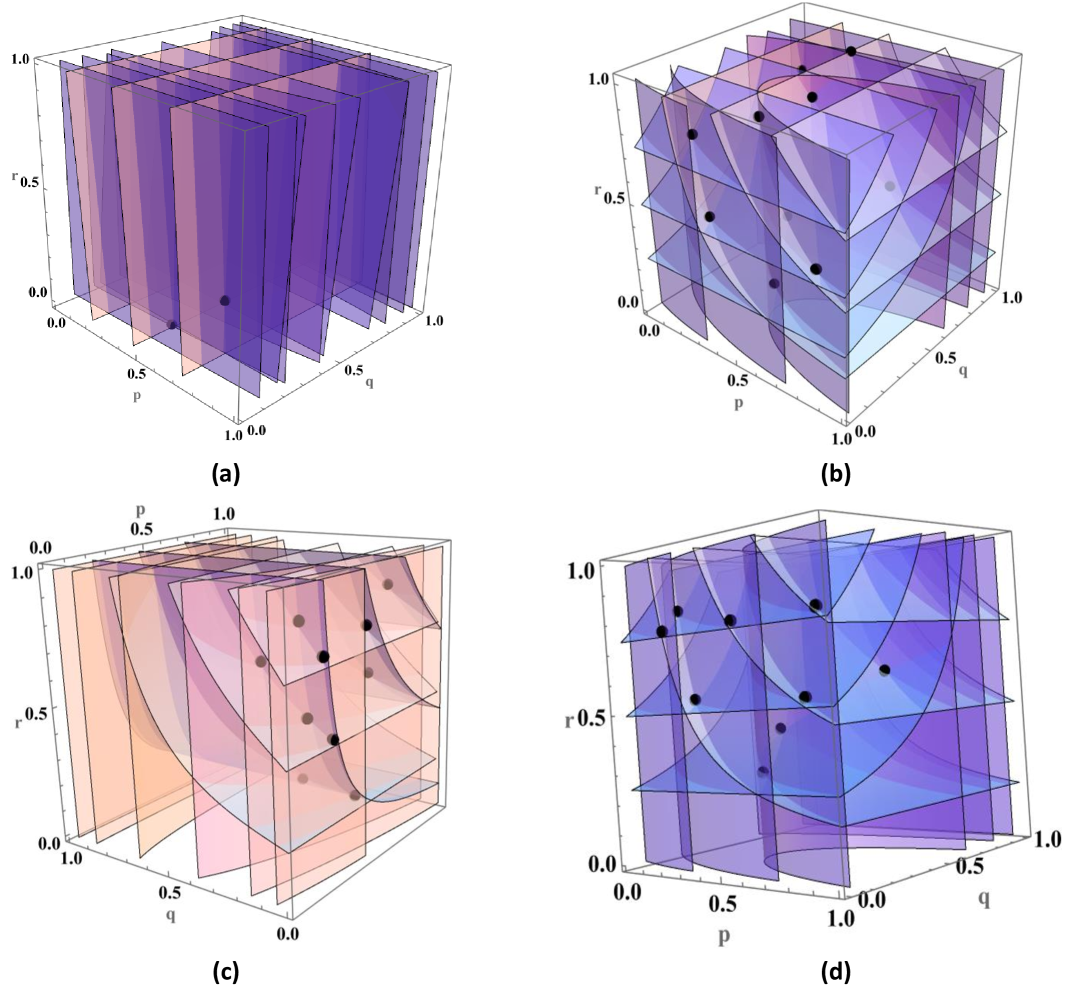
\n ## 3D Surface Plots in a Unit Cube ### Overview The image displays four separate 3D plots, labeled (a), (b), (c), and (d), arranged in a 2x2 grid. Each plot visualizes semi-transparent, colored surfaces and scattered black data points within a cubic domain defined by three axes: `p`, `q`, and `r`. All axes range from 0.0 to 1.0. The plots appear to be generated by mathematical software (e.g., Mathematica, MATLAB) and likely represent different functions, manifolds, or solution sets within a unit cube. ### Components/Axes * **Axes Labels:** Each plot has three axes labeled `p`, `q`, and `r`. * **Axis Scales:** All axes are linear and span the interval [0.0, 1.0]. Tick marks are visible at 0.0, 0.5, and 1.0. * **Subplot Labels:** Each plot is identified by a lowercase letter in parentheses: `(a)`, `(b)`, `(c)`, `(d)`, placed directly below its respective cube. * **Visual Elements:** * **Surfaces:** Multiple semi-transparent, colored surfaces are plotted within each cube. Colors include shades of purple, blue, and pink/peach. The surfaces vary in shape from planar to complexly curved. * **Data Points:** Solid black spheres (points) are scattered within the volume of each cube. Their number and distribution differ per plot. * **Legend:** There is no explicit legend provided. The meaning of the different surface colors and the data points is not defined within the image itself. ### Detailed Analysis **Subplot (a):** * **Surface Geometry:** The surfaces appear as a series of parallel, vertical planes. They are oriented perpendicular to the `p`-axis, meaning they represent constant values of `p`. The planes are spaced at regular intervals along the `p`-axis. * **Surface Color:** The planes are colored in a gradient from light pink/peach (near `p=0`) to dark purple (near `p=1`). * **Data Points:** Two black data points are visible. One is located near the center of the cube (approximately `p=0.5, q=0.5, r=0.5`). The second is positioned lower and closer to the front face (approximately `p=0.7, q=0.3, r=0.2`). **Subplot (b):** * **Surface Geometry:** The surfaces are complex, intersecting, and curved. They do not align with constant coordinate planes. The shapes suggest they could be level sets of a multivariate function or solutions to a system of equations. * **Surface Color:** The surfaces are predominantly shades of purple and blue, with some pinkish hues visible where surfaces overlap or are viewed edge-on. * **Data Points:** Approximately 10-12 black data points are scattered throughout the volume. They do not appear to lie on the visible surfaces. Their distribution seems somewhat random, with a slight clustering in the upper half of the cube (higher `r` values). **Subplot (c):** * **Surface Geometry:** The surfaces are curved and appear to "drape" from the top face (`r=1`) of the cube downwards. They are not closed shapes but rather open sheets. The curvature is more pronounced along the `q` and `r` dimensions. * **Surface Color:** The surfaces are primarily light pink/peach, with some purple/blue areas where they intersect or are viewed from a different angle. * **Data Points:** Approximately 8-10 black data points are visible. They are mostly located in the central region of the cube, seemingly "caught" between or near the draped surfaces. **Subplot (d):** * **Surface Geometry:** This plot features a prominent, central, bowl-shaped or saddle-shaped surface that is open at the top. Additional, more planar surfaces intersect this central shape. * **Surface Color:** The central curved surface is a distinct blue. The intersecting planar surfaces are shades of purple. * **Data Points:** Approximately 7-9 black data points are present. They are distributed around the central blue surface, with several points appearing to lie on or very close to the purple planar surfaces. ### Key Observations 1. **Progression of Complexity:** There is a clear visual progression from the simple, planar geometry in (a) to the increasingly complex, curved, and intersecting geometries in (b), (c), and (d). 2. **Point-Surface Relationship:** The relationship between the black data points and the colored surfaces varies. In (a), points are isolated from the planes. In (c) and (d), points appear more associated with the surfaces, potentially lying on them or in their vicinity. 3. **Color Consistency:** While the specific meaning is unknown, the color palette (purple, blue, pink) is used consistently across all four subplots, suggesting they may represent related mathematical entities or parameters. 4. **Viewpoint:** All four cubes are viewed from the same isometric perspective, with the origin (`p=0, q=0, r=0`) at the bottom-left-rear corner. This allows for direct visual comparison of the geometries. ### Interpretation The image likely illustrates different scenarios or solutions within a three-parameter space (`p`, `q`, `r`), common in fields like optimization, statistical mechanics, game theory, or control systems. * **What the data suggests:** The plots demonstrate how the structure of a solution set (the colored surfaces) and the location of specific points of interest (the black dots) can change dramatically under different conditions or for different functions. * **Plot (a)** could represent a simple, decoupled system where one variable (`p`) is independent, creating planar constraints. * **Plots (b), (c), and (d)** show increasingly coupled and nonlinear relationships between the variables, resulting in complex manifolds. * **How elements relate:** The black points are likely specific samples, optima, equilibria, or initial conditions being studied in relation to the broader solution landscape defined by the surfaces. Their placement relative to the surfaces is the key piece of information. * **Notable patterns/anomalies:** The most striking pattern is the transformation of the surface topology. The transition from parallel planes to a complex, interconnected web of curved sheets indicates a fundamental change in the underlying mathematical model. The consistent use of color implies a categorical distinction (e.g., different constraint types, energy levels, or probability thresholds) that is not labeled but is maintained across all visualizations. **In summary, this figure is a technical visualization comparing four distinct 3D manifolds within a unit cube, each populated with a set of data points. It serves to contrast the geometric complexity and point distribution across different models or parameter sets.**