## Graph Evolution Diagram: Network State at Different Time Steps ### Overview The image shows a network diagram evolving through three time steps (t=0, t=1, t=2). The network consists of nodes (numbered 0-9) and edges (represented by lines). The nodes are colored either red or green. The edges are generally yellow, but some edges are highlighted in blue or magenta to indicate changes between time steps. Numerical values are associated with some edges in the first time step. ### Components/Axes * **Nodes:** Numbered 0 through 9, represented by circles. Node colors are either red or green. * **Edges:** Represented by yellow lines connecting the nodes. Some edges are highlighted in blue or magenta. * **Time Steps:** Three distinct network states labeled as t=0, t=1, and t=2. * **Edge Weights (t=0):** Numerical values associated with some edges in the first time step. * **Highlighted Edges:** A blue edge labeled 'q' in t=1 and a magenta edge labeled 'p' in t=2. ### Detailed Analysis **Time Step t=0:** * Nodes 0, 1, 2, 3, and 4 are red. * Nodes 5, 6, 7, 8, and 9 are green. * Edge weights are present for some edges: * Edge between nodes 4 and 8: 1.62 * Edge between nodes 4 and 2: 1.32 * Edge between nodes 8 and 5: 2.25 * Edge between nodes 5 and 9: 1.71 * Edge between nodes 7 and 8: 1.92 * Edge between nodes 9 and 1: 2.38 * Edge between nodes 3 and 0: 1.45 * Edge between nodes 0 and 6: 1.1 * Edge between nodes 6 and 9: 1.84 * Edge between nodes 1 and 6: 1.13 **Time Step t=1:** * Nodes 0, 1, 2, and 4 are red. * Nodes 3, 5, 6, 7, 8, and 9 are green. * A blue edge labeled 'q' connects nodes 3 and 7. **Time Step t=2:** * Nodes 0, 1, 2, 4, and 8 are red. * Nodes 3, 5, 6, 7, and 9 are green. * A magenta edge labeled 'p' connects nodes 4 and 8. ### Key Observations * The network structure remains generally consistent across the three time steps, but the node colors change. * At t=1, node 3 changes from red to green. * At t=2, node 8 changes from green to red. * The highlighted edges (blue 'q' and magenta 'p') indicate specific changes or events occurring in the network. * The edge weights are only present at t=0. ### Interpretation The diagram illustrates the evolution of a network where nodes can change their state (represented by color). The highlighted edges 'q' and 'p' likely represent specific interactions or events that trigger the state changes in nodes 3 and 8, respectively. The edge weights at t=0 could represent the initial strength or importance of connections within the network. The change in node colors suggests a dynamic process occurring within the network, possibly representing the spread of information, influence, or some other property. The absence of edge weights at t=1 and t=2 suggests that these values are either not relevant or are changing over time.

\n ## Diagram: Network Evolution over Time ### Overview The image presents a series of three network diagrams illustrating the evolution of a network over three time steps (t=0, t=1, and t=2). The network consists of nine nodes, labeled 1 through 9, connected by edges. Each edge is labeled with a numerical value, presumably representing a weight or distance. The diagrams show how the network connections change over time, with some edges appearing, disappearing, or changing their weights. ### Components/Axes The diagrams do not have traditional axes. They consist of nodes (circles) and edges (lines) connecting the nodes. Each edge has a numerical label. The time step is indicated below each diagram (t=0, t=1, t=2). At t=2, two edges are highlighted in different colors: a purple edge labeled 'p' and a blue edge labeled 'q'. ### Detailed Analysis or Content Details **t = 0:** * Nodes: 1, 2, 3, 4, 5, 6, 7, 8, 9 * Edges and Weights: * 1-6: 1.84 * 1-9: 1.13 * 2-4: 1.62 * 2-8: 1.32 * 3-1: 1.45 * 3-7: 1.92 * 4-2: 1.62 * 4-8: 2.25 * 5-8: 1.71 * 5-9: 2.38 * 6-1: 1.84 * 7-3: 1.92 * 7-9: 2.38 * 8-2: 1.32 * 8-4: 2.25 * 8-5: 1.71 * 9-5: 2.38 * 9-7: 2.38 * 9-1: 1.13 **t = 1:** * Nodes: 1, 2, 3, 4, 5, 6, 7, 8, 9 * Edges and Weights: * 1-6: 1.84 * 1-9: 1.13 * 2-4: 1.62 * 2-8: 1.32 * 3-7: 1.92 * 4-2: 1.62 * 4-8: 2.25 * 5-8: 1.71 * 5-9: 2.38 * 6-1: 1.84 * 7-3: 1.92 * 7-9: 2.38 * 8-2: 1.32 * 8-4: 2.25 * 8-5: 1.71 * 9-5: 2.38 * 9-7: 2.38 * 3-7: 1.92 (new edge) * 3-7: 1.92 * 3-7: 1.92 * Highlighted Edge: * 3-7: q (blue) **t = 2:** * Nodes: 1, 2, 3, 4, 5, 6, 7, 8, 9 * Edges and Weights: * 1-6: 1.84 * 1-9: 1.13 * 2-4: 1.62 * 2-8: 1.32 * 3-1: 1.45 * 4-2: 1.62 * 4-8: 2.25 * 5-8: 1.71 * 5-9: 2.38 * 6-1: 1.84 * 7-3: 1.92 * 7-9: 2.38 * 8-2: 1.32 * 8-4: 2.25 * 8-5: 1.71 * 9-5: 2.38 * 9-7: 2.38 * Highlighted Edges: * 3-7: q (blue) * 4-8: p (purple) ### Key Observations * The network appears to be relatively stable between t=0 and t=1, with only the addition of the edge 3-7. * At t=2, the network returns to a configuration similar to t=0, but with the edges 3-7 and 4-8 highlighted. * The edge weights remain constant throughout the three time steps. * The highlighted edges 'p' and 'q' at t=2 suggest these edges are of particular interest or are involved in a specific process. ### Interpretation The diagrams likely represent a dynamic network where connections are formed and potentially broken over time. The edge weights could represent distances, costs, or strengths of relationships between nodes. The evolution from t=0 to t=1 shows the addition of a connection between nodes 3 and 7. The return to a similar configuration at t=2, with the highlighting of edges 'p' and 'q', could indicate a cyclical process or a specific path being emphasized. The highlighting of edges 'p' and 'q' at t=2 suggests these edges are important for a particular analysis. They might represent critical paths, bottlenecks, or edges involved in a specific event. The network's evolution could be modeling a communication network, a transportation system, or a social network, where connections represent interactions or relationships. The cyclical nature of the changes suggests a dynamic equilibrium or a repeating pattern. The diagram is a visual representation of a network's state at different points in time, allowing for the analysis of its evolution and the identification of key features.

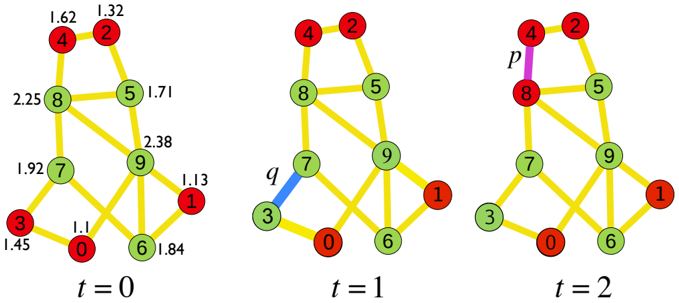
## Network Diagram: Temporal Evolution of a Weighted Graph (t=0, t=1, t=2) ### Overview The image displays three network graphs arranged horizontally, representing the state of the same graph at three sequential time steps, labeled `t=0`, `t=1`, and `t=2`. The graph consists of 10 nodes (numbered 0 through 9) connected by edges. The primary changes across time steps are the highlighting of specific edges with distinct colors and labels, while the underlying graph structure and node states remain constant. ### Components/Axes * **Time Step Labels:** Located at the bottom center of each respective graph: `t = 0`, `t = 1`, `t = 2`. * **Nodes:** 10 circular nodes, each containing a unique integer identifier from 0 to 9. * **Node Colors:** Nodes are colored either red or green. The color assignment is consistent across all three time steps. * **Red Nodes:** 0, 1, 2, 3, 4 * **Green Nodes:** 5, 6, 7, 8, 9 * **Edges:** Lines connecting nodes. The base color for all edges is yellow. * **Edge Annotations (Time-Specific):** * At `t=1`: The edge connecting node 3 and node 7 is colored **blue** and labeled with the letter **`q`**. * At `t=2`: The edge connecting node 4 and node 8 is colored **purple** and labeled with the letter **`p`**. * **Numerical Labels (Present only at t=0):** Several nodes have a decimal number placed adjacent to them, likely representing an initial weight, value, or metric. * Node 4: `1.62` * Node 2: `1.32` * Node 8: `2.25` * Node 5: `1.71` * Node 7: `1.92` * Node 9: `2.38` * Node 3: `1.45` * Node 0: `1.1` * Node 1: `1.13` * Node 6: `1.84` ### Detailed Analysis **Graph Structure (Constant across t=0, t=1, t=2):** The graph's topology is fixed. The nodes are arranged in a rough, irregular grid. The connections (edges) are as follows: * Node 0 is connected to nodes 3, 6, and 7. * Node 1 is connected to nodes 6 and 9. * Node 2 is connected to nodes 4 and 5. * Node 3 is connected to nodes 0 and 7. * Node 4 is connected to nodes 2 and 8. * Node 5 is connected to nodes 2, 8, and 9. * Node 6 is connected to nodes 0, 1, and 9. * Node 7 is connected to nodes 0, 3, 8, and 9. * Node 8 is connected to nodes 4, 5, and 7. * Node 9 is connected to nodes 1, 5, 6, and 7. **Temporal Progression:** 1. **t=0:** The initial state. All edges are yellow. Nine of the ten nodes have an associated numerical value. 2. **t=1:** The state after one time step. The only visual change is the edge between nodes 3 and 7, which is now blue and labeled `q`. All numerical values from t=0 are absent. 3. **t=2:** The state after two time steps. The blue edge `q` from t=1 reverts to yellow. A new change occurs: the edge between nodes 4 and 8 is now purple and labeled `p`. ### Key Observations 1. **Stable Core:** The graph's structure (which nodes connect to which) and the classification of nodes (red vs. green) do not change over time. 2. **Transient Highlighting:** The annotations (`p` and `q`) and their associated edge colors are specific to a single time step. They appear to mark events or operations occurring at that step. 3. **Initial Data:** The numerical values are only present at the initial time step (`t=0`), suggesting they are starting conditions or inputs that are processed or transformed in subsequent steps. 4. **Spatial Consistency:** The physical layout of the nodes is identical in all three diagrams, allowing for direct visual comparison of the changing edge highlights. ### Interpretation This diagram likely illustrates the execution of a graph algorithm or a dynamic process on a network over discrete time steps. * **What the data suggests:** The process involves identifying or operating on specific edges at each step. The labels `p` and `q` could represent variables, weights, or the names of operations (e.g., "process edge p"). The initial numerical values at `t=0` might be node potentials, costs, or scores that influence which edges (`p` and `q`) are selected for action at `t=1` and `t=2`. * **How elements relate:** The red/green node dichotomy could represent two states (e.g., active/inactive, infected/susceptible, source/target). The algorithm appears to act on edges connecting nodes of different states or based on the initial numerical values. The fact that the highlighted edge changes from `q` (between a red node 3 and green node 7) to `p` (between a red node 4 and green node 8) suggests a sequential or iterative selection criterion. * **Notable patterns/anomalies:** The most significant pattern is the shift in focus from one edge (`q`) to another (`p`). This is not random; it follows the graph's structure. An anomaly is the absence of any numerical data after `t=0`, implying the process is not about updating those numbers visually, but perhaps using them to drive the edge selection shown. The diagram prioritizes showing *which* edge is active at each step over showing continuous value updates. **In summary, the image is a technical schematic for a time-variant graph process, emphasizing the sequential selection of specific edges (`q` then `p`) from an initial weighted state, within a stable network of two node types.**

## Network Diagram: Dynamic Node Connections Over Time ### Overview The image depicts a dynamic network system visualized across three time steps (t=0, t=1, t=2). Nodes are represented as colored circles (red, green, orange) with numerical labels, connected by weighted edges. The diagrams show progressive changes in connectivity and node states over time. ### Components/Axes - **Nodes**: Labeled 0-9, colored red (high priority), green (active), or orange (neutral). - **Edges**: Weighted connections with numerical values (e.g., 1.62, 2.25). - **Time Steps**: - **t=0**: Initial network state with dense connectivity. - **t=1**: Intermediate state with partial edge removal/addition. - **t=2**: Final state with further edge modifications. - **Highlighted Edges**: - **Blue edge** (t=1): Connects nodes 3 and 7. - **Purple edge** (t=2): Connects nodes 4 and 8. ### Detailed Analysis #### t=0 (Initial State) - **Nodes**: - Red: 0, 1, 2, 3, 4 (high-priority nodes). - Green: 5, 6, 7, 8, 9 (active nodes). - **Edges**: - Highest weight: 2.38 (node 9 to 6). - Lowest weight: 1.1 (node 0 to 3). - Notable cluster: Nodes 0-3-7-9 form a dense subnetwork. #### t=1 (Intermediate State) - **Changes**: - Edge between nodes 3 and 0 removed. - New blue edge added between nodes 3 and 7 (weight: 1.84). - Node 3 turns orange (neutral state). - **Edge Weights**: - Remaining highest weight: 2.25 (node 8 to 5). - New edge weight: 1.84 (node 3 to 7). #### t=2 (Final State) - **Changes**: - Blue edge (3-7) removed. - Purple edge added between nodes 4 and 8 (weight: 1.32). - Node 4 turns red (high-priority). - **Edge Weights**: - Highest weight: 2.38 (node 9 to 6, unchanged). - New edge weight: 1.32 (node 4 to 8). ### Key Observations 1. **Dynamic Connectivity**: - Edges are added/removed over time, suggesting a reconfiguration process. - The purple edge (4-8) at t=2 may represent a critical new connection. 2. **Node State Transitions**: - Node 3 shifts from green (active) to orange (neutral) at t=1. - Node 4 transitions to red (high-priority) at t=2. 3. **Weight Trends**: - Edge weights fluctuate but remain within a narrow range (1.1–2.38). - The 1.84 edge (3-7) at t=1 is the only intermediate-weight connection. ### Interpretation This diagram likely models a **dynamic system** where nodes represent entities (e.g., servers, agents) and edges represent interactions or dependencies. The time steps suggest: - **t=0**: Initial setup with maximum connectivity. - **t=1**: Optimization phase, removing redundant edges (3-0) and introducing a new pathway (3-7). - **t=2**: Final optimization, prioritizing high-value nodes (4, 8) and reinforcing critical connections (4-8). The numerical weights may reflect **efficiency metrics** (e.g., latency, cost) or **strength of interactions**. The highlighted edges (blue/purple) could denote **critical transitions** or **emergent pathways** in the system. The color-coded nodes imply a **hierarchical structure**, with red nodes acting as central hubs. **Notable Anomaly**: The persistence of the 2.38 edge (9-6) across all time steps suggests it is a **stable, high-priority connection** resistant to reconfiguration.