## Network Diagram: Dynamic Node Connections Over Time
### Overview
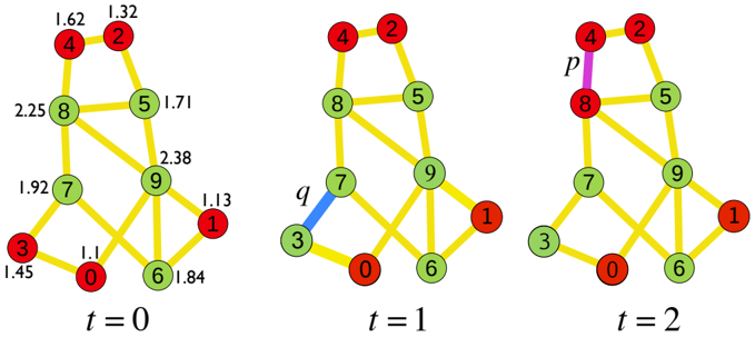
The image depicts a dynamic network system visualized across three time steps (t=0, t=1, t=2). Nodes are represented as colored circles (red, green, orange) with numerical labels, connected by weighted edges. The diagrams show progressive changes in connectivity and node states over time.
### Components/Axes
- **Nodes**: Labeled 0-9, colored red (high priority), green (active), or orange (neutral).
- **Edges**: Weighted connections with numerical values (e.g., 1.62, 2.25).
- **Time Steps**:
- **t=0**: Initial network state with dense connectivity.
- **t=1**: Intermediate state with partial edge removal/addition.
- **t=2**: Final state with further edge modifications.
- **Highlighted Edges**:
- **Blue edge** (t=1): Connects nodes 3 and 7.
- **Purple edge** (t=2): Connects nodes 4 and 8.
### Detailed Analysis
#### t=0 (Initial State)
- **Nodes**:
- Red: 0, 1, 2, 3, 4 (high-priority nodes).
- Green: 5, 6, 7, 8, 9 (active nodes).
- **Edges**:
- Highest weight: 2.38 (node 9 to 6).
- Lowest weight: 1.1 (node 0 to 3).
- Notable cluster: Nodes 0-3-7-9 form a dense subnetwork.
#### t=1 (Intermediate State)
- **Changes**:
- Edge between nodes 3 and 0 removed.
- New blue edge added between nodes 3 and 7 (weight: 1.84).
- Node 3 turns orange (neutral state).
- **Edge Weights**:
- Remaining highest weight: 2.25 (node 8 to 5).
- New edge weight: 1.84 (node 3 to 7).
#### t=2 (Final State)
- **Changes**:
- Blue edge (3-7) removed.
- Purple edge added between nodes 4 and 8 (weight: 1.32).
- Node 4 turns red (high-priority).
- **Edge Weights**:
- Highest weight: 2.38 (node 9 to 6, unchanged).
- New edge weight: 1.32 (node 4 to 8).
### Key Observations
1. **Dynamic Connectivity**:
- Edges are added/removed over time, suggesting a reconfiguration process.
- The purple edge (4-8) at t=2 may represent a critical new connection.
2. **Node State Transitions**:
- Node 3 shifts from green (active) to orange (neutral) at t=1.
- Node 4 transitions to red (high-priority) at t=2.
3. **Weight Trends**:
- Edge weights fluctuate but remain within a narrow range (1.1–2.38).
- The 1.84 edge (3-7) at t=1 is the only intermediate-weight connection.
### Interpretation
This diagram likely models a **dynamic system** where nodes represent entities (e.g., servers, agents) and edges represent interactions or dependencies. The time steps suggest:
- **t=0**: Initial setup with maximum connectivity.
- **t=1**: Optimization phase, removing redundant edges (3-0) and introducing a new pathway (3-7).
- **t=2**: Final optimization, prioritizing high-value nodes (4, 8) and reinforcing critical connections (4-8).
The numerical weights may reflect **efficiency metrics** (e.g., latency, cost) or **strength of interactions**. The highlighted edges (blue/purple) could denote **critical transitions** or **emergent pathways** in the system. The color-coded nodes imply a **hierarchical structure**, with red nodes acting as central hubs.
**Notable Anomaly**: The persistence of the 2.38 edge (9-6) across all time steps suggests it is a **stable, high-priority connection** resistant to reconfiguration.