## Circuit Diagram and Correlation Graph: Component Interactions and Temporal Correlations
### Overview
The image contains two primary components:
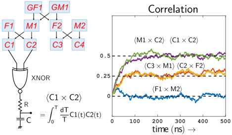
1. A **circuit diagram** on the left depicting a logic gate (XNOR) connected to multiple components labeled with identifiers (e.g., GF1, GM1, F1, M1, etc.).
2. A **correlation graph** on the right showing time-dependent correlation values for pairwise interactions between components (e.g., ⟨M1 × C2⟩, ⟨C1 × C2⟩).
---
### Components/Axes
#### Circuit Diagram
- **Labels**:
- Top layer: `GF1`, `GM1` (green boxes).
- Middle layer: `F1`, `M1`, `F2`, `M2` (blue boxes).
- Bottom layer: `C1`, `C2`, `C3`, `C4` (red boxes).
- **Connections**:
- `GF1` and `GM1` feed into `M1` and `M2`.
- `F1` and `F2` feed into `C1` and `C2`.
- `C1` and `C2` connect to an XNOR gate via resistors (`R`) and capacitors (`C`).
- **Equation**:
- `⟨C1 × C2⟩ = ∫₀ᵀ (dT/T)C1(t)C2(t)` (integral of normalized product of C1 and C2 over time).
#### Correlation Graph
- **Axes**:
- **X-axis**: Time (ns), ranging from 0 to 500 ns.
- **Y-axis**: Correlation (unitless), ranging from 0 to 0.5.
- **Legend**:
- **Colors and Labels**:
- Green: `⟨M1 × C2⟩`
- Purple: `⟨C1 × C2⟩`
- Orange: `⟨C3 × M1⟩`
- Red: `⟨C2 × F2⟩`
- Blue: `⟨F1 × M2⟩`
- **Dashed Reference Lines**:
- Horizontal lines at 0.5, 0.25, and 0.
---
### Detailed Analysis
#### Correlation Graph Trends
1. **Green Line (`⟨M1 × C2⟩`)**:
- Peaks at ~0.55 at ~150 ns, then oscillates around 0.5.
- Crosses the 0.5 threshold twice.
2. **Purple Line (`⟨C1 × C2⟩`)**:
- Starts at 0, rises steadily to ~0.45 by 500 ns.
- Smooth, monotonic increase.
3. **Orange Line (`⟨C3 × M1⟩`)**:
- Fluctuates between 0.2 and 0.35.
- No clear trend; irregular oscillations.
4. **Red Line (`⟨C2 × F2⟩`)**:
- Peaks at ~0.3 at ~200 ns, then declines to ~0.15 by 500 ns.
5. **Blue Line (`⟨F1 × M2⟩`)**:
- Remains below 0.25 throughout.
- Sharp dip to ~0.1 at ~300 ns.
#### Circuit Diagram Observations
- The XNOR gate integrates signals from `C1` and `C2`, with the equation suggesting a time-averaged product correlation.
- Components are hierarchically organized: `GF1`/`GM1` (top) → `F1`/`F2`/`M1`/`M2` (middle) → `C1`/`C2`/`C3`/`C4` (bottom).
---
### Key Observations
1. **High Correlation**:
- `⟨M1 × C2⟩` and `⟨C1 × C2⟩` show the strongest correlations, suggesting critical interactions between memory (`M1`) and capacitor (`C2`) components.
2. **Decaying Correlations**:
- `⟨C2 × F2⟩` and `⟨F1 × M2⟩` exhibit lower or decaying values, indicating weaker or transient relationships.
3. **Stability**:
- `⟨C3 × M1⟩` remains stable but low, possibly reflecting a secondary interaction.
---
### Interpretation
1. **System Behavior**:
- The correlation graph reveals that interactions between memory (`M1`, `M2`) and capacitor (`C1`, `C2`) components dominate the system’s behavior. The XNOR gate’s output (`⟨C1 × C2⟩`) correlates with the product of `C1` and `C2`, aligning with the integral equation.
2. **Temporal Dynamics**:
- Peaks in `⟨M1 × C2⟩` at 150 ns suggest a transient event (e.g., signal propagation delay or feedback loop).
- The steady rise in `⟨C1 × C2⟩` implies a cumulative effect of capacitor interactions over time.
3. **Anomalies**:
- The blue line (`⟨F1 × M2⟩`) remains consistently low, potentially indicating a design limitation or unoptimized coupling between `F1` and `M2`.
---
### Conclusion
The data demonstrates that the system’s performance is heavily influenced by the interplay between memory and capacitor components. The XNOR gate’s role in integrating `C1` and `C2` signals is critical, as evidenced by the strong correlation trends. Further optimization of `F1`/`M2` coupling could enhance overall system efficiency.