\n
## Heatmap: Classification Accuracies
### Overview
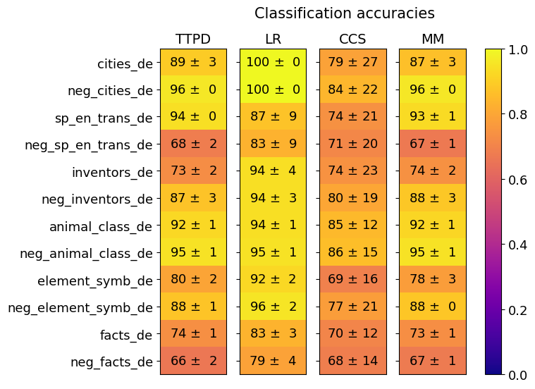
The image is a heatmap titled "Classification accuracies" that displays the performance (accuracy scores with standard deviations) of four different methods (TTPD, LR, CCS, MM) across twelve distinct datasets. The data is presented in a grid where rows represent datasets and columns represent methods. Each cell contains a numerical accuracy value (mean ± standard deviation) and is color-coded based on the accuracy score, with a color scale bar provided on the right.
### Components/Axes
* **Title:** "Classification accuracies" (top center).
* **Column Headers (Methods):** TTPD, LR, CCS, MM (top row, from left to right).
* **Row Labels (Datasets):** Listed vertically on the left side. From top to bottom:
1. `cities_de`
2. `neg_cities_de`
3. `sp_en_trans_de`
4. `neg_sp_en_trans_de`
5. `inventors_de`
6. `neg_inventors_de`
7. `animal_class_de`
8. `neg_animal_class_de`
9. `element_symb_de`
10. `neg_element_symb_de`
11. `facts_de`
12. `neg_facts_de`
* **Color Scale/Legend:** Positioned vertically on the far right. It is a gradient bar ranging from 0.0 (dark purple/blue) at the bottom to 1.0 (bright yellow) at the top. Major tick marks are at 0.0, 0.2, 0.4, 0.6, 0.8, and 1.0. The color indicates the accuracy value within each cell.
* **Data Cells:** A 12-row by 4-column grid. Each cell contains text in the format "XX ± Y", where XX is the mean accuracy and Y is the standard deviation. The background color of each cell corresponds to the mean accuracy value according to the color scale.
### Detailed Analysis
**Data Extraction (Row by Row):**
1. **cities_de:**
* TTPD: 89 ± 3 (Yellow-orange)
* LR: 100 ± 0 (Bright yellow)
* CCS: 79 ± 27 (Orange, high variance)
* MM: 87 ± 3 (Yellow-orange)
2. **neg_cities_de:**
* TTPD: 96 ± 0 (Yellow)
* LR: 100 ± 0 (Bright yellow)
* CCS: 84 ± 22 (Orange-yellow, high variance)
* MM: 96 ± 0 (Yellow)
3. **sp_en_trans_de:**
* TTPD: 94 ± 0 (Yellow)
* LR: 87 ± 9 (Yellow-orange)
* CCS: 74 ± 21 (Orange, high variance)
* MM: 93 ± 1 (Yellow)
4. **neg_sp_en_trans_de:**
* TTPD: 68 ± 2 (Orange-red)
* LR: 83 ± 9 (Yellow-orange)
* CCS: 71 ± 20 (Orange, high variance)
* MM: 67 ± 1 (Orange-red)
5. **inventors_de:**
* TTPD: 73 ± 2 (Orange)
* LR: 94 ± 4 (Yellow)
* CCS: 74 ± 23 (Orange, high variance)
* MM: 74 ± 2 (Orange)
6. **neg_inventors_de:**
* TTPD: 87 ± 3 (Yellow-orange)
* LR: 94 ± 3 (Yellow)
* CCS: 80 ± 19 (Orange-yellow, high variance)
* MM: 88 ± 3 (Yellow-orange)
7. **animal_class_de:**
* TTPD: 92 ± 1 (Yellow)
* LR: 94 ± 1 (Yellow)
* CCS: 85 ± 12 (Yellow-orange, moderate variance)
* MM: 92 ± 1 (Yellow)
8. **neg_animal_class_de:**
* TTPD: 95 ± 1 (Yellow)
* LR: 95 ± 1 (Yellow)
* CCS: 86 ± 15 (Yellow-orange, moderate variance)
* MM: 95 ± 1 (Yellow)
9. **element_symb_de:**
* TTPD: 80 ± 2 (Orange-yellow)
* LR: 92 ± 2 (Yellow)
* CCS: 69 ± 16 (Orange, high variance)
* MM: 78 ± 3 (Orange-yellow)
10. **neg_element_symb_de:**
* TTPD: 88 ± 1 (Yellow-orange)
* LR: 96 ± 2 (Yellow)
* CCS: 77 ± 21 (Orange, high variance)
* MM: 88 ± 0 (Yellow-orange)
11. **facts_de:**
* TTPD: 74 ± 1 (Orange)
* LR: 83 ± 3 (Yellow-orange)
* CCS: 70 ± 12 (Orange, moderate variance)
* MM: 73 ± 1 (Orange)
12. **neg_facts_de:**
* TTPD: 66 ± 2 (Orange-red)
* LR: 79 ± 4 (Orange-yellow)
* CCS: 68 ± 14 (Orange, moderate variance)
* MM: 67 ± 1 (Orange-red)
### Key Observations
1. **Method Performance:** The **LR** method consistently achieves the highest or near-highest accuracy across all datasets, with perfect scores (100 ± 0) on `cities_de` and `neg_cities_de`. It rarely has a standard deviation above 9.
2. **Dataset Difficulty:** The datasets `neg_sp_en_trans_de` and `neg_facts_de` appear to be the most challenging, with the lowest accuracies across all methods (mostly in the 60s and 70s). The `neg_` prefix variants do not uniformly perform worse than their positive counterparts; for example, `neg_cities_de` scores are very high.
3. **Variance:** The **CCS** method exhibits the highest variance (standard deviations often in the teens or twenties), indicating its performance is less consistent across different runs or folds compared to the other methods.
4. **Color Correlation:** The color coding accurately reflects the numerical values. Bright yellow cells (e.g., LR on `cities_de`) correspond to 1.0, while the darkest orange-red cells (e.g., TTPD on `neg_facts_de`) correspond to values in the mid-0.6 range.
5. **TTPD vs. MM:** These two methods often have similar performance levels, with TTPD sometimes having a slight edge (e.g., on `sp_en_trans_de`) and MM sometimes having a slight edge (e.g., on `neg_inventors_de`).
### Interpretation
This heatmap provides a comparative analysis of four classification methods on a suite of German-language (`_de` suffix) datasets, likely related to specific tasks (city names, translations, inventors, animal classification, element symbols, general facts) and their negated or contrastive versions (`neg_` prefix).
The data suggests that the **LR (Logistic Regression?)** method is the most robust and accurate for these particular tasks, achieving top performance with high consistency. The **CCS** method, while sometimes competitive in mean accuracy, is unreliable due to its high variance. The performance drop on `neg_sp_en_trans_de` and `neg_facts_de` might indicate these datasets contain more ambiguous, complex, or noisy examples that are harder for all models to classify correctly.
The near-perfect scores on the `cities_de` datasets by LR suggest this task may be relatively straightforward for that model, possibly due to clear, distinctive features in the data. The comparison between standard and `neg_` datasets could be used to analyze model robustness to data perturbations or to understand the nature of the classification boundary. Overall, the visualization effectively communicates that method choice significantly impacts both accuracy and reliability across this domain.